<?xml version="1.0" encoding="utf-8"?><feed xmlns="http://www.w3.org/2005/Atom" ><generator uri="https://jekyllrb.com/" version="3.10.0">Jekyll</generator><link href="https://jhkook30.github.io/feed.xml" rel="self" type="application/atom+xml" /><link href="https://jhkook30.github.io/" rel="alternate" type="text/html" /><updated>2026-09-24T19:02:05+09:00</updated><id>https://jhkook30.github.io/feed.xml</id><title type="html">Home</title><subtitle>Researcher at Sejong University, working on privacy-preserving and verifiable machine learning — training on data that cannot be shared, and proving what a model did without revealing it.</subtitle><author><name>Jihyung Kook (국지형)</name><email>jhkook30@gmail.com</email></author><entry><title type="html">II. Post-quantum Cryptography: B-4. GLWE Cryptosystem</title><link href="https://jhkook30.github.io/posts/2026/05/he-note-04/" rel="alternate" type="text/html" title="II. Post-quantum Cryptography: B-4. GLWE Cryptosystem" /><published>2026-05-11T00:00:00+09:00</published><updated>2026-05-11T00:00:00+09:00</updated><id>https://jhkook30.github.io/posts/2026/05/he-note-04</id><content type="html" xml:base="https://jhkook30.github.io/posts/2026/05/he-note-04/"><![CDATA[<!-- 배너 이미지 + 링크 -->
<p><a href="https://arxiv.org/abs/2503.05136" target="_blank">
  <img src="/images/explorations/he-book/he-book-cover.png" alt="The Beginner's Textbook for Fully Homomorphic Encryption (by Ronny Ko)" style="max-width:500px; width:100%; border-radius:10px; margin:20px auto; display:block;" />
</a></p>

<p>This post is based on <em>The Beginner’s Textbook for Fully Homomorphic Encryption</em> by <strong>Ronny Ko</strong>.<br />
In this post, I provide a summary and review of <strong>“II. Post-quantum Cryptography: B-4. GLWE Cryptosystem.”</strong></p>

<hr />

<!--more-->

<h1 id="b-4-glwe-cryptosystem">B-4. GLWE Cryptosystem</h1>

<p>The GLWE cryptosystem is a <strong>generalized form</strong> to encompass both the LWE and RLWE cryptosystems.</p>

<h3 id="1-key-notations">1. Key Notations</h3>

<p>Like in LWE and RLWE, a new public key $A$ is created for each ciphertext,<br />
whereas the same secret key $S$ is used for all ciphertexts.</p>

<p>The GLWE ciphertext is defined as a tuple $({A_i}_{i=0}^{k-1}, B)$, where</p>

\[B = \sum_{i=0}^{k-1}(A_i \cdot S_i) + \Delta \cdot M + E\]

<table>
  <thead>
    <tr>
      <th>Symbol</th>
      <th>Meaning</th>
    </tr>
  </thead>
  <tbody>
    <tr>
      <td>$A_i \in R_{n,q}^k$, for $i = 0, \ldots, k-1$</td>
      <td>Public polynomials (freshly sampled per ciphertext)</td>
    </tr>
    <tr>
      <td>$S_i \in R_{n,2}^k$, for $i = 0, \ldots, k-1$</td>
      <td>Secret polynomials (fixed)</td>
    </tr>
    <tr>
      <td>$M \in R_{n,t}$, where $t &lt; q$ and $t \mid q$</td>
      <td>Message polynomial</td>
    </tr>
    <tr>
      <td>$E \leftarrow \chi_\sigma$</td>
      <td>Noise polynomial sampled from Gaussian distribution</td>
    </tr>
  </tbody>
</table>

<h3 id="2-relation-to-lwe-and-rlwe">2. Relation to LWE and RLWE</h3>

<p>GLWE generalizes both LWE and RLWE through its parameters $n$ and $k$:</p>

<table>
  <thead>
    <tr>
      <th>Cryptosystem</th>
      <th>Parameter Setting</th>
      <th>Secret Key</th>
    </tr>
  </thead>
  <tbody>
    <tr>
      <td><strong>LWE</strong></td>
      <td>$n = 1$ (degree-0 polynomials = scalars)</td>
      <td>$k$ scalar constants forming a vector</td>
    </tr>
    <tr>
      <td><strong>RLWE</strong></td>
      <td>$k = 1$ (single polynomial)</td>
      <td>One $(n-1)$-degree polynomial $S_0$</td>
    </tr>
    <tr>
      <td><strong>GLWE</strong></td>
      <td>General $n, k$</td>
      <td>$k$ polynomials of degree $(n-1)$</td>
    </tr>
  </tbody>
</table>

<p>👉 LWE and RLWE are special cases of GLWE — GLWE unifies them under a single framework.</p>

<h2 id="b-41-setup">B-4.1 Setup</h2>

<p>To be continued …</p>

<!--  
Let $t$ be the size of the plaintext space, and $q$ the size of the ciphertext space,  
where $t < q$ and $t \mid q$.
 
### 1. Secret Key
 
Randomly sample a list of $k$ polynomials:
 
$$
\{S_i\}_{i=0}^{k-1} \xleftarrow{\$} R_{n,2}^k
$$
 
- Each $S_i$ is an $(n-1)$-degree polynomial
- Each coefficient is a binary value in $\{0, 1\}$
→ Unlike RLWE (which encodes $n$ secret coefficients in one polynomial),  
GLWE encodes $n \cdot k$ secret coefficients total across $k$ polynomials.
 
### 2. Scaling Factor
 
$$
\Delta = \left\lfloor \frac{q}{t} \right\rfloor
$$
 
---
 
## B-4.2 Encryption
 
### 1. Encryption Steps
 
1) Suppose we have a plaintext polynomial:
$$
M \in R_{n,t}
$$
2) Sample a list of $k$ random polynomials as a one-time public key:
$$
\{A_i\}_{i=0}^{k-1} \xleftarrow{\$} R_{n,q}^k
$$
3) Sample a small noise polynomial:
$$
E \xleftarrow{\chi_\sigma} R_{n,q}
$$
→ Each of the $n$ coefficients is a small number in $\mathbb{Z}_q$
4) Scale the plaintext:
$$
\Delta \cdot M \in R_{n,q}
$$
👉 Since $M \in R_{n,t}$ and $\Delta = \frac{q}{t}$, each coefficient satisfies $0 \le \Delta \cdot m_i < q$
 
5) Compute:
$$
B = \sum_{i=0}^{k-1}(A_i \cdot S_i) + \Delta \cdot M + E \;\; \in R_{n,q}
$$
6) Final ciphertext:
$$
(\{A_i\}_{i=0}^{k-1}, B)
$$
<details>
  <summary>
    <span style="font-size:1em; font-weight:bold;">
      🔐 Summary B-4.2: GLWE Encryption
    </span>
  </summary>
  <div markdown="1" style="
    border:2px solid #007acc;
    border-radius:10px;
    padding:16px;
    background:#f0f8ff;
    margin-top:10px;
  ">
### Initial Setup
 
$$
\Delta = \left\lfloor \frac{q}{t} \right\rfloor, \quad \{S_i\}_{i=0}^{k-1} \xleftarrow{\$} R_{n,2}^k
$$
 
### Encryption Input
 
$$
M \in R_{n,t}, \quad \{A_i\}_{i=0}^{k-1} \xleftarrow{\$} R_{n,q}^k, \quad E \xleftarrow{\chi_\sigma} R_{n,q}
$$
 
### Encryption Steps
 
1. Scale up $M \longrightarrow \Delta M \in R_{n,q}$
2. Compute $B = \displaystyle\sum_{i=0}^{k-1}(A_i \cdot S_i) + \Delta M + E \in R_{n,q}$
3. Output $GLWE_{S,\sigma}(\Delta M) = (\{A_i\}_{i=0}^{k-1}, B) \in R_{n,q}^{k+1}$
  </div>
</details>
---
 
## B-4.3 Decryption
 
### 1. Decryption Steps
 
1) Given the ciphertext $(\{A_i\}_{i=0}^{k-1}, B)$, remove the secret-dependent term:
$$
B - \sum_{i=0}^{k-1}(A_i \cdot S_i) = \Delta \cdot M + E
$$
 
2) Round each coefficient of $\Delta M + E$ to the nearest multiple of $\Delta$:
$$
\left\lfloor \Delta M + E \right\rceil_{\Delta}
$$
 
👉 This successfully eliminates $E$, provided each noise coefficient $e_i$ satisfies:
$$
|e_i| < \frac{\Delta}{2}
$$
 
3) Recover the plaintext by scaling down:
$$
M = \frac{\left\lfloor \Delta M + E \right\rceil_{\Delta}}{\Delta} \bmod t \;\; \in R_{n,t}
$$
 
→ Equivalent to right-shifting each coefficient by $\log_2 \Delta$ bits
 
<details>
  <summary>
    <span style="font-size:1em; font-weight:600;">
      🔐 Summary B-4.3: GLWE Decryption
    </span>
  </summary>
  <div markdown="1" style="
    border:2px solid #007acc;
    border-radius:10px;
    padding:16px;
    background:#f0f8ff;
    margin-top:10px;
  ">
### Decryption Input
 
$$
C = (\{A_i\}_{i=0}^{k-1}, B) \in R_{n,q}^{k+1}
$$
 
### Decryption Steps
 
1. Remove the secret term:
$$
GLWE^{-1}_{S,\sigma}(C) = B - \sum_{i=0}^{k-1}(A_i \cdot S_i) = \Delta M + E \in R_{n,q}
$$
2. Scale down:
$$
\left\lfloor \frac{\Delta M + E}{\Delta} \right\rceil \bmod t = M \in R_{n,t}
$$
### Correctness Condition
 
$$
|e_i| < \frac{\Delta}{2}
$$
 
→ Ensures correct rounding and successful decryption
 
  </div>
</details>
---
 
## B-4.3.1 Discussion
 
**1. Size of $n$:**  
A large $n$ increases the number of secret key coefficient terms in each $S_i$, making it harder to guess the complete secret key. Also, higher-degree polynomials can encode more plaintext terms in $M$, improving throughput efficiency.
 
**2. Size of $k$:**  
A large $k$ increases the number of secret key polynomials $(S_0, S_1, \cdots, S_k)$ and one-time public key polynomials $(A_0, A_1, \cdots, A_k)$, making it harder for an attacker to guess the complete secret keys.  
👉 Meanwhile, there is always a single $M$ and $E$ per GLWE ciphertext, regardless of $k$.
 
**3. Reducing the Ciphertext Size:**  
The public key $\{A_i\}_{i=0}^{k-1}$ must be freshly created for each ciphertext, which can be large. To reduce this, each ciphertext can instead include a seed $d$ for a pseudo-random number generation hash function $H$, so the public key is computed on-the-fly as $\{H(d), H(H(d)), H(H(H(d))), \cdots\}$.
 
---
 
## B-4.4 An Alternative Version of GLWE
 
An alternative version of (Summary B-4.2), where the **sign of each $A_i S_i$ is flipped**:
 
<details>
  <summary>
    <span style="font-size:1em; font-weight:bold;">
      🔄 Summary B-4.4: Alternative GLWE Cryptosystem
    </span>
  </summary>
  <div markdown="1" style="
    border:2px solid #6a0dad;
    border-radius:10px;
    padding:16px;
    background:#f5f0ff;
    margin-top:10px;
  ">
### Initial Setup
 
$$
\Delta = \left\lfloor \frac{q}{t} \right\rfloor, \quad \{S_i\}_{i=0}^{k-1} \xleftarrow{\$} R_{n,2}^k
$$
 
### Encryption Input
 
$$
M \in R_{n,t}, \quad \{A_i\}_{i=0}^{k-1} \xleftarrow{\$} R_{n,q}^k, \quad E \xleftarrow{\chi_\sigma} R_{n,q}
$$
 
1. Scale up $M \longrightarrow \Delta M \in R_{n,q}$
2. Compute $B = -\displaystyle\sum_{i=0}^{k-1}(A_i \cdot S_i) + \Delta M + E \in R_{n,q}$
3. $GLWE_{S,\sigma}(\Delta M) = (\{A_i\}_{i=0}^{k-1}, B) \in R_{n,q}^{k+1}$
### Decryption Input
 
$$
C = (\{A_i\}_{i=0}^{k-1}, B) \in R_{n,q}^{k+1}
$$
 
1. $GLWE^{-1}_{S,\sigma}(C) = B + \displaystyle\sum_{i=0}^{k-1}(A_i \cdot S_i) = \Delta M + E \in R_{n,q}$
2. Scale down $\left\lfloor \dfrac{\Delta M + E}{\Delta} \right\rceil = M \in R_{n,t}$
For correct decryption, every noise coefficient $e_i$ should be: $e_i < \dfrac{\Delta}{2}$.
 
  </div>
</details>
👉 Even if the $A_i S_i$ terms flip their signs, the decryption stage cancels them out by **adding** their equivalent double-sign-flipped terms; thus, the same correctness of decryption is preserved.
 
---
 
## B-4.5 Public Key Encryption
 
In §B-4.2, it is assumed that the **secret key owner** encrypts each plaintext.  
This section explains a **public key encryption scheme**, where anyone who knows the public key can encrypt — but only the secret key owner can decrypt.
 
The high-level idea is that a portion of the encryption components is pre-computed at setup and published as a public key. At encryption time, the public key is multiplied by an additional randomness $U$ and combined with additional noises $(E_1, E_2)$ to create unpredictable randomness in each ciphertext.
 
<details>
  <summary>
    <span style="font-size:1em; font-weight:bold;">
      🔑 Summary B-4.5: GLWE Public Key Encryption
    </span>
  </summary>
  <div markdown="1" style="
    border:2px solid #007acc;
    border-radius:10px;
    padding:16px;
    background:#f0f8ff;
    margin-top:10px;
  ">
### Initial Setup
 
- Scaling factor: $\Delta = \left\lfloor \dfrac{q}{t} \right\rfloor$
- Secret key: $\{S_i\}_{i=0}^{k-1} \xleftarrow{\$} R_{n,2}^k$
- Public key pair $(PK_1, PK_2) \in R_{n,q}^{k+1}$ generated as:
$$
\bar{A} = \{A_i\}_{i=0}^{k-1} \xleftarrow{\$} R_{n,q}^k, \quad E \xleftarrow{\sigma} R_{n,q}
$$
 
$$
PK_1 = \bar{A} \cdot \bar{S} + E \in R_{n,q}
$$
 
$$
PK_2 = \bar{A} \in R_{n,q}^k
$$
 
### Encryption Input
 
$$
M \in R_{n,t}, \quad U \xleftarrow{\$} R_{n,2}, \quad E_1 \xleftarrow{\sigma} R_{n,q}, \quad E_2 \xleftarrow{\sigma} R_{n,q}^k
$$
 
1. Scale up $M \longrightarrow \Delta M \in R_{n,q}$
2. Compute:
$$
B = PK_1 \cdot U + \Delta M + E_1 \in R_{n,q}
$$
$$
D = PK_2 \cdot U + E_2 \in R_{n,q}^k
$$
3. $GLWE_{S,\sigma}(\Delta M) = (D, B) \in R_{n,q}^{k+1}$
### Decryption Input
 
$$
C = (D, B) \in R_{n,q}^{k+1}
$$
 
1. $GLWE^{-1}_{S,\sigma}(C) = B - D \cdot \bar{S} = \Delta M + E_{all} \in R_{n,q}$
2. Scale down $\left\lfloor \dfrac{\Delta M + E_{all}}{\Delta} \right\rceil = M \in R_{n,t}$
For correct decryption, every noise coefficient $e_i$ of $E_{all}$ should be: $e_i < \dfrac{\Delta}{2}$.
 
  </div>
</details>
### Derivation of Decryption Correctness
 
$$
GLWE^{-1}_{S,\sigma}(C = (B, D)) = B - D \cdot \bar{S}
$$
 
$$
= (PK_1 \cdot U + \Delta M + E_1) - (PK_2 \cdot U + E_2) \cdot \bar{S}
$$
 
$$
= (\bar{A} \cdot \bar{S} + E) \cdot U + \Delta M + E_1 - (\bar{A} \cdot U) \cdot \bar{S} - E_2 \cdot \bar{S}
$$
 
$$
= \Delta M + E \cdot U + E_1 - E_2 \cdot \bar{S}
$$
 
$$
= \Delta M + E_{all} \quad \text{where } E_{all} = E \cdot U + E_1 - E_2 \cdot \bar{S}
$$ -->]]></content><author><name>Jihyung Kook (국지형)</name><email>jhkook30@gmail.com</email></author><category term="cryptography" /><category term="post-quantum-cryptography" /><category term="lattice-based-cryptography" /><category term="glwe" /><summary type="html"><![CDATA[This post is based on The Beginner’s Textbook for Fully Homomorphic Encryption by Ronny Ko. In this post, I provide a summary and review of “II. Post-quantum Cryptography: B-4. GLWE Cryptosystem.”]]></summary></entry><entry><title type="html">II. Post-quantum Cryptography: B-3. RLWE Cryptosystem</title><link href="https://jhkook30.github.io/posts/2026/04/he-note-03/" rel="alternate" type="text/html" title="II. Post-quantum Cryptography: B-3. RLWE Cryptosystem" /><published>2026-04-03T00:00:00+09:00</published><updated>2026-04-03T00:00:00+09:00</updated><id>https://jhkook30.github.io/posts/2026/04/he-note-03</id><content type="html" xml:base="https://jhkook30.github.io/posts/2026/04/he-note-03/"><![CDATA[<!-- 배너 이미지 + 링크 -->
<p><a href="https://arxiv.org/abs/2503.05136" target="_blank">
  <img src="/images/explorations/he-book/he-book-cover.png" alt="The Beginner's Textbook for Fully Homomorphic Encryption (by Ronny Ko)" style="max-width:500px; width:100%; border-radius:10px; margin:20px auto; display:block;" />
</a></p>

<p>This post is based on <em>The Beginner’s Textbook for Fully Homomorphic Encryption</em> by <strong>Ronny Ko</strong>.<br />
In this post, I provide a summary and review of <strong>“II. Post-quantum Cryptography: B-3. RLWE Cryptosystem.”</strong></p>

<hr />

<!--more-->

<h1 id="b-3-rlwe-cryptosystem">B-3. RLWE Cryptosystem</h1>

<h3 id="1-key-notations">1. Key Notations</h3>

<p>Like in LWE, a new public key $A$ is created for each ciphertext,<br />
whereas the same secret key $S$ is used for all ciphertexts.</p>

<p>In RLWE, all polynomials are computed in the ring:
\(R_{n,q} = \mathbb{Z}_q[x] / (x^n + 1)\)</p>

<ul>
  <li>$x^n + 1$ is a cyclotomic polynomial</li>
  <li>$n = 2^f$ for some integer $f$</li>
  <li>Coefficients are in $\mathbb{Z}_q$</li>
</ul>

<p>In RLWE, the ciphertext is defined as a tuple $(A, B)$, where
\(B = S \cdot A + \Delta \cdot M + E\)</p>

<table>
  <thead>
    <tr>
      <th>Symbol</th>
      <th>Meaning</th>
      <th> </th>
    </tr>
  </thead>
  <tbody>
    <tr>
      <td>$(A, B) \in R_{n,q} \times R_{n,q}$</td>
      <td>Ciphertext</td>
      <td> </td>
    </tr>
    <tr>
      <td>$A \in_R R_{n,q}$</td>
      <td>Public polynomial (freshly sampled per ciphertext)</td>
      <td> </td>
    </tr>
    <tr>
      <td>$S \in_R R_{n,q}$</td>
      <td>Secret polynomial (fixed)</td>
      <td> </td>
    </tr>
    <tr>
      <td>$M \in R_{n,t}$, where $t&lt;q$ and $t</td>
      <td>q$</td>
      <td>Message polynomial</td>
    </tr>
    <tr>
      <td>$E \leftarrow \chi$</td>
      <td>Noise polynomial sampled from error distribution</td>
      <td> </td>
    </tr>
  </tbody>
</table>

<h3 id="2-notes">2. Notes</h3>

<ul>
  <li>Each element in $R_{n,q}$ is a polynomial of degree at most $n-1$</li>
  <li>$M$ is often defined in:
\(R_t = \mathbb{Z}_t[x]/(x^n + 1)\)
and scaled using $\Delta = \frac{q}{t}$</li>
</ul>

<h2 id="b-31-setup">B-3.1 Setup</h2>

<p>Let $t$ be the size of the plaintext space, and $q$ the size of the ciphertext space, where $t &lt; q$ and $t \mid q$.</p>

<h3 id="1-secret-key">1. Secret Key</h3>

<p>Randomly sample a polynomial:
\(S \leftarrow R_{n,2}\)</p>

<ul>
  <li>$S$ is a polynomial of degree at most $n-1$</li>
  <li>Each coefficient is a binary value in ${0,1}$</li>
</ul>

<p>→ This means $S$ encodes $n$ secret coefficients</p>

<h3 id="2-scaling-factor">2. Scaling Factor</h3>

<p>Define the scaling factor:
\(\Delta = \left\lfloor \frac{q}{t} \right\rfloor\)</p>

<p>→ This is used to map plaintext from a smaller space into the ciphertext space</p>

<h3 id="3-relation-to-lwe">3. Relation to LWE</h3>

<p>RLWE setup is similar to LWE, with one key difference:</p>

<ul>
  <li>
    <p>LWE:
\(S \in \mathbb{Z}_2^k \quad (\text{vector})\)</p>
  </li>
  <li>
    <p>RLWE:
\(S \in R_{n,2} \quad (\text{polynomial})\)</p>
  </li>
</ul>

<p>→ Instead of a vector of length $k$,<br />
$S$ is an $(n-1)$-degree polynomial encoding $n$ secret coefficients</p>

<h2 id="b-32-encryption">B-3.2 Encryption</h2>

<h3 id="1-encryption-steps">1. Encryption Steps</h3>

<p>1) Suppose we have a plaintext polynomial:
\(M \in R_{n,t}\)
→ coefficients represent the plaintext values</p>

<p>2) Sample a random polynomial:
\(A \in_R R_{n,q}\)
→ This acts as a one-time public component</p>

<p>3) Sample a small noise polynomial:
\(E \leftarrow \chi\)
→ coefficients are small (e.g., Gaussian noise)</p>

<p>4) Scale the plaintext:
\(\Delta \cdot M\)
→ This embeds $M$ into the ciphertext space $R_{n,q}$</p>

<p>👉 Since $M \in R_{n,t}$ and $\Delta = \frac{q}{t}$,</p>

<ul>
  <li>each coefficient of $M$ is in $[0, t)$</li>
  <li>after scaling:</li>
</ul>

\[0 \le \Delta \cdot M &lt; q\]

<p>→ Thus, $\Delta M \in R_{n,q}$</p>

<p>5) Compute the ciphertext:
\(B = A \cdot S + \Delta \cdot M + E \;\; \in R_{n,q}\)</p>

<p>6) Final ciphertext:
\((A, B)\)</p>

<details>
  <summary>
    <span style="font-size:1em; font-weight:bold;">
      🔐 Summary B-3.2: RLWE Encryption
    </span>
  </summary>

  <div style="
    border:2px solid #007acc;
    border-radius:10px;
    padding:16px;
    background:#f0f8ff;
    margin-top:10px;
  ">

    <h3 id="initial-setup">1. Initial Setup</h3>

    <ul>
      <li>
        <p>Work in the ring:
\(R_{n,q} = \mathbb{Z}_q[x]/(x^n + 1)\)</p>
      </li>
      <li>$\Delta = \frac{q}{t}$, where $t \mid q$ (i.e., $q = t \cdot k$ for some integer $k$)</li>
      <li>$S \leftarrow R_{n,2}$, which means each coefficient of $S$ is binary (in ${0,1}$), not that the modulus is 2</li>
    </ul>

    <hr />

    <h3 id="encryption-input">2. Encryption Input</h3>

\[M \in R_{n,t}, \quad
A \in_R R_{n,q}, \quad
E \xleftarrow{\chi_\sigma} R_{n,q}\]

    <hr />

    <h3 id="encryption-steps">3. Encryption Steps</h3>

    <ol>
      <li>
        <p>Scale the plaintext:
\(\Delta \cdot M \in R_{n,q}\)</p>
      </li>
      <li>
        <p>Compute:
\(B = A \cdot S + \Delta \cdot M + E \pmod{R_{n,q}}\)</p>
      </li>
      <li>
        <p>Output ciphertext:
\(RLWE_{S,\sigma}(\Delta M) = (A, B) \in R_{n,q}^2\)</p>
      </li>
    </ol>

  </div>
</details>

<h2 id="b-33-decryption">B-3.3 Decryption</h2>

<h3 id="1-decryption-steps">1. Decryption Steps</h3>

<p>1) Given a ciphertext $(A, B)$, where</p>

\[B = A \cdot S + \Delta \cdot M + E \;\; \in R_{n,q}\]

<p>2) Remove the secret-dependent term:</p>

\[B - A \cdot S = \Delta \cdot M + E\]

<p>3) Recover the scaled message by rounding:</p>

\[\left\lfloor \Delta \cdot M + E \right\rceil_{\Delta}\]

<p>→ Round each coefficient to the nearest multiple of $\Delta$</p>

<p>👉 If each coefficient of $E$ satisfies:
\(|e_i| &lt; \frac{\Delta}{2}\)</p>

<p>then:
\(\left\lfloor \Delta M + E \right\rceil_{\Delta} = \Delta M\)</p>

<p>4) Recover the plaintext:</p>

\[M = \frac{1}{\Delta} \cdot \left\lfloor \Delta M + E \right\rceil_{\Delta}\]

<p>→ equivalent to right-shifting each coefficient by $\log_2 \Delta$ bits</p>

<details>
  <summary>
    <span style="font-size:1em; font-weight:600;">
      🔐 Summary B-3.3: RLWE Decryption
    </span>
  </summary>

  <div style="
    border:2px solid #007acc;
    border-radius:10px;
    padding:16px;
    background:#f0f8ff;
    margin-top:10px;
  ">

    <h3 id="decryption-input">1. Decryption Input</h3>

\[C = (A, B) \in R_{n,q}^2\]

    <h3 id="decryption-steps">2. Decryption Steps</h3>

    <ol>
      <li>
        <p>Remove the secret term:
\(B - A \cdot S = \Delta M + E \pmod{R_{n,q}}\)</p>
      </li>
      <li>
        <p>Scale down:
\(\frac{\left\lfloor \Delta M + E \right\rceil_{\Delta}}{\Delta}
\;\; \bmod t
= M \in R_{n,t}\)</p>
      </li>
    </ol>

    <h3 id="correctness-condition">3. Correctness Condition</h3>

\[|e_i| &lt; \frac{\Delta}{2}\]

    <p>→ Ensures correct rounding and successful decryption</p>

    <p>→ If $t \nmid q$, $q$ should be sufficiently larger than $t$ to avoid decryption errors</p>

  </div>
</details>]]></content><author><name>Jihyung Kook (국지형)</name><email>jhkook30@gmail.com</email></author><category term="cryptography" /><category term="post-quantum-cryptography" /><category term="lattice-based-cryptography" /><category term="rlwe" /><summary type="html"><![CDATA[This post is based on The Beginner’s Textbook for Fully Homomorphic Encryption by Ronny Ko. In this post, I provide a summary and review of “II. Post-quantum Cryptography: B-3. RLWE Cryptosystem.”]]></summary></entry><entry><title type="html">II. Post-quantum Cryptography: B-2. LWE Cryptosystem</title><link href="https://jhkook30.github.io/posts/2026/04/he-note-02/" rel="alternate" type="text/html" title="II. Post-quantum Cryptography: B-2. LWE Cryptosystem" /><published>2026-04-01T00:00:00+09:00</published><updated>2026-04-01T00:00:00+09:00</updated><id>https://jhkook30.github.io/posts/2026/04/he-note-02</id><content type="html" xml:base="https://jhkook30.github.io/posts/2026/04/he-note-02/"><![CDATA[<!-- 배너 이미지 + 링크 -->
<p><a href="https://arxiv.org/abs/2503.05136" target="_blank">
  <img src="/images/explorations/he-book/he-book-cover.png" alt="The Beginner's Textbook for Fully Homomorphic Encryption (by Ronny Ko)" style="max-width:500px; width:100%; border-radius:10px; margin:20px auto; display:block;" />
</a></p>

<p>This post is based on <em>The Beginner’s Textbook for Fully Homomorphic Encryption</em> by <strong>Ronny Ko</strong>.<br />
In this post, I provide a summary and review of <strong>“II. Post-quantum Cryptography: B-2. LWE Cryptosystem.”</strong></p>

<hr />

<!--more-->

<h1 id="b-2-lwe-cryptosystem">B-2. LWE Cryptosystem</h1>

<h2 id="b-21-setup">B-2.1 Setup</h2>

<h3 id="key-notations">Key Notations</h3>

<table>
  <thead>
    <tr>
      <th>Symbol</th>
      <th>Meaning</th>
    </tr>
  </thead>
  <tbody>
    <tr>
      <td>$[0, t)$</td>
      <td>Plaintext Range</td>
    </tr>
    <tr>
      <td>$[0, q)$, where $t&lt;q$</td>
      <td>Ciphertext Range ($t$ is much smaller than $q$)</td>
    </tr>
    <tr>
      <td>$S \in_R \mathbb{Z}_2^k$</td>
      <td>Secret key sampled uniformly at random (each entry in ${0,1}$)</td>
    </tr>
    <tr>
      <td>$\Delta = \frac{q}{t}$</td>
      <td>Scaling factor of plaintext</td>
    </tr>
  </tbody>
</table>

<h2 id="b-22-encryption">B-2.2 Encryption</h2>

<h3 id="1-encryption-steps">1. Encryption Steps</h3>

<p>1) Suppose we have a plaintext $m \in \mathbb{Z}_t$</p>

<p>2) Sample a random vector $A \in_R \mathbb{Z}_q^k$<br />
   → This acts as a one-time public key</p>

<p>3) Sample a small noise $e \in \mathbb{Z}_q$</p>

<p>→ $e \xleftarrow{\chi_\sigma} Z_{q}$ (Gaussian noise)</p>

<p>4) Scale the plaintext:
\(\Delta \cdot m\)
→ This embeds $m$ into the ciphertext space $\mathbb{Z}_q$</p>

<p>👉 Since $m \in [0, t)$ and $\Delta = \frac{q}{t}$,</p>

\[\Delta m = \frac{q}{t} \cdot m \le \frac{q}{t}(t-1) = q - \frac{q}{t}\]

<p>→ Therefore,
\(0 \le \Delta m &lt; q\)</p>

<p>→ Thus, $\Delta m \in \mathbb{Z}_q$</p>

<p>5) Compute the ciphertext:
   \(b = A \cdot S  + \Delta \cdot m + e \;\; \in \mathbb{Z}_q\)</p>

<h3 id="2-final-form">2. Final Form</h3>

<p>The LWE ciphertext is:
\((A, b)\)</p>

<details>
  <summary>
    <span style="font-size:1em; font-weight:bold;">
      🔐 Summary B-2.2: LWE Encryption
    </span>
  </summary>

  <div style="
    border:2px solid #007acc;
    border-radius:10px;
    padding:16px;
    background:#f0f8ff;
    margin-top:10px;
  ">

    <h3 id="initial-setup">1. Initial Setup</h3>

    <ul>
      <li>$\Delta = \frac{q}{t}$, where $t$ divides $q$</li>
      <li>$S \in_R \mathbb{Z}_2^k$</li>
    </ul>

    <h3 id="encryption-input">2. Encryption Input</h3>

\[m \in \mathbb{Z}_t,\quad
A \in_R \mathbb{Z}_q^k,\quad
e \xleftarrow{\chi_\sigma} Z_{q}\]

    <h3 id="encryption-steps">3. Encryption Steps</h3>

    <ol>
      <li>
        <p>Scale the plaintext:
\(\Delta \cdot m \in \mathbb{Z}_q\)</p>
      </li>
      <li>
        <p>Compute:
\(b = A \cdot S + \Delta \cdot m + e \pmod{q}\)</p>
      </li>
      <li>
        <p>Output ciphertext:
\(LWE_{S,\sigma}(\Delta m) = (A, b) \in \mathbb{Z}_q^{k+1}\)</p>
      </li>
    </ol>

  </div>
</details>

<h2 id="b-23-decryption">B-2.3 Decryption</h2>

<h3 id="1-decryption-steps">1. Decryption Steps</h3>

<p>1) Given a ciphertext $(A, b)$, where</p>

\[b = A \cdot S + \Delta \cdot m + e \;\; \in \mathbb{Z}_q\]

<p>2) Remove the secret-dependent term:</p>

\[b - A \cdot S = \Delta \cdot m + e\]

<p>3) Recover the scaled message by rounding:</p>

\[\left\lfloor \Delta \cdot m + e \right\rceil_{\Delta}\]

<p>→ Round to the nearest multiple of $\Delta$</p>

<p>👉 If $|e| &lt; \frac{\Delta}{2}$, then:
\(\left\lfloor \Delta m + e \right\rceil_{\Delta} = \Delta m\)</p>

<p>4) Recover the plaintext:</p>

\[m = \frac{1}{\Delta} \cdot \left\lfloor \Delta m + e \right\rceil_{\Delta} = \frac{1}{\Delta} \cdot \Delta m = m\]

<details>
  <summary>
    <span style="font-size:1em; font-weight:600;">
      🔐 Summary B-2.3: LWE Decryption
    </span>
  </summary>

  <div style="
    border:2px solid #007acc;
    border-radius:10px;
    padding:16px;
    background:#f0f8ff;
    margin-top:10px;
  ">

    <h3 id="decryption-input">1. Decryption Input</h3>

\[C = (A, b) \in \mathbb{Z}_q^{k+1}\]

    <h3 id="decryption-steps">2. Decryption Steps</h3>

    <ol>
      <li>
        <p>Remove the secret term:
\(b - A \cdot S = \Delta m + e \pmod{q}\)</p>
      </li>
      <li>
        <p>Scale down:
\(\frac{\left\lfloor \Delta m + e \right\rceil_{\Delta}}{\Delta} \;\; \bmod t
= m \in \mathbb{Z}_t\)</p>
      </li>
    </ol>

    <h3 id="correctness-condition">3. Correctness Condition</h3>

\[e &lt; \frac{\Delta}{2}\]

    <p>→ Ensures correct rounding and successful decryption</p>

  </div>
</details>

<h3 id="2-why-scaling-by-delta">2. Why Scaling by $\Delta$?</h3>

<p>Scaling by $\Delta = \frac{q}{t}$ separates the plaintext and noise:</p>

<ul>
  <li>Multiplying by $\Delta$ shifts $m$ to higher bits (by $\log_2 \Delta$ bits)</li>
  <li>The noise $e$ remains in the lower bits</li>
</ul>

<p>During decryption,
\(\frac{\Delta m + e}{\Delta} = m + \frac{e}{\Delta}\)</p>

<p>This effectively shifts the value back (right-shift), removing the noise through rounding.</p>

<p>👉 If $e$ is small, rounding recovers $m$ correctly.</p>

<details>
  <summary>
    <span style="font-size:1em; font-weight:600;">
      B-2.3.1. In the Case of $t$ not Dividing $q$
    </span>
  </summary>

  <div style="
    border:2px solid #007acc;
    border-radius:10px;
    padding:16px;
    background:#f0f8ff;
    margin-top:10px;
  ">

    <h3 id="setting">1. Setting</h3>

    <p>Now suppose that $t$ does <strong>not</strong> divide $q$.</p>

    <p>Then we set the scaling factor as:</p>

\[\Delta = \left\lfloor \frac{q}{t} \right\rfloor\]

    <p>→ Even if $m &gt; t$, decryption still correctly recovers the result. <strong>But why?</strong></p>

    <h3 id="writing-the-plaintext-as-a-wrapped-value">2. Writing the plaintext as a wrapped value</h3>

    <p>To analyze this, we write the plaintext $m$ as</p>

\[m = m' + kt, \quad m' \in \mathbb{Z}_t,\; k \in \mathbb{Z}\]

    <p>Here, $m’$ is the actual value of $m$ modulo $t$, and $kt$ represents how many times $m$ has wrapped around modulo $t$.</p>

    <p>So the goal of decryption is really to recover $m’ = m \bmod t$.</p>

    <h3 id="expanding-the-scaled-plaintext">3. Expanding the scaled plaintext</h3>

    <p>The scaled plaintext with noise is</p>

\[\left\lfloor \frac{q}{t} \right\rfloor m + e\]

    <p>Substituting $m = m’ + kt$, we get</p>

\[\left\lfloor \frac{q}{t} \right\rfloor m + e
=
\left\lfloor \frac{q}{t} \right\rfloor m'
+
\left\lfloor \frac{q}{t} \right\rfloor kt
+
e\]

    <p>Now focus on the second term:</p>

\[\left\lfloor \frac{q}{t} \right\rfloor kt\]

    <p>Since</p>

\[\frac{q}{t}
=
\left\lfloor \frac{q}{t} \right\rfloor
+
\left(\frac{q}{t} - \left\lfloor \frac{q}{t} \right\rfloor\right),\]

    <p>we can rewrite it as</p>

\[\left\lfloor \frac{q}{t} \right\rfloor kt
=
\frac{q}{t}kt
-
\left(\frac{q}{t} - \left\lfloor \frac{q}{t} \right\rfloor\right)kt\]

    <p>Because</p>

\[\frac{q}{t}kt = qk,\]

    <p>this becomes</p>

\[\left\lfloor \frac{q}{t} \right\rfloor kt
=
qk
-
\left(\frac{q}{t} - \left\lfloor \frac{q}{t} \right\rfloor\right)kt\]

    <p>Therefore,</p>

\[\left\lfloor \frac{q}{t} \right\rfloor m + e
=
\left\lfloor \frac{q}{t} \right\rfloor m'
+
qk
-
\left(\frac{q}{t} - \left\lfloor \frac{q}{t} \right\rfloor\right)kt
+
e\]

    <h3 id="what-happens-modulo-q">4. What happens modulo $q$?</h3>

    <p>$qk$ is a multiple of $q$, so under modulo $q$ it disappears:</p>

\[qk \equiv 0 \pmod q\]

    <p>So after reduction modulo $q$, the expression behaves like</p>

\[\left\lfloor \frac{q}{t} \right\rfloor m'
-
\left(\frac{q}{t} - \left\lfloor \frac{q}{t} \right\rfloor\right)kt
+
e\]

    <p>That means the wrap-around part $kt$ does <strong>not</strong> remain as plaintext.<br />
Instead, it gets absorbed into an additional error term.</p>

    <h3 id="why-is-the-extra-error-small">5. Why is the extra error small?</h3>

    <p>Since</p>

\[0 \le
\frac{q}{t} - \left\lfloor \frac{q}{t} \right\rfloor
&lt; 1,\]

    <p>we have</p>

\[0 \le
\left(\frac{q}{t} - \left\lfloor \frac{q}{t} \right\rfloor\right)kt
&lt; kt\]

    <p>So this extra term is strictly smaller than $kt$.</p>

    <p>The text therefore treats this part as an overestimated noise term and writes the expression conceptually as</p>

\[\Delta m + e = \left\lfloor \frac{q}{t} \right\rfloor m + e 
\;\approx\; 
\left\lfloor \frac{q}{t} \right\rfloor m'
+
qk
-
e'
+
e,\]

    <p>where $e’ = kt$ is used as an upper bound, since the extra term is strictly smaller than $kt$.</p>

    <p>In other words, the wrap-around portion of $m$ does not destroy correctness.<br />
It only contributes some bounded extra noise.</p>

    <h3 id="decryption">6. Decryption</h3>

    <p>Recall the LWE decryption relation:</p>

\[b - A \cdot S \bmod q = \Delta m + e\]

    <p>Using the rewritten form above,</p>

\[\Delta m + e
\;\approx\;
\left\lfloor \frac{q}{t} \right\rfloor m' + qk - e' + e
\pmod q\]

    <p>Now divide by $\left\lfloor \frac{q}{t} \right\rfloor$ and reduce modulo $t$:</p>

\[\left[
\frac{1}{\left\lfloor q/t \right\rfloor}
\cdot
\left(
\left\lfloor \frac{q}{t} \right\rfloor m' + qk - e' + e
\;\bmod q
\right)
\right]
\bmod t\]

    <h3 id="simplifying-the-expression">7. Simplifying the expression</h3>

    <p>Since $qk \equiv 0 \pmod q$, the $qk$ term disappears:</p>

\[\left[
\frac{1}{\left\lfloor q/t \right\rfloor}
\cdot
\left(
\left\lfloor \frac{q}{t} \right\rfloor m' - e' + e
\right)
\right]
\bmod t\]

    <p>Now divide by $\left\lfloor q/t \right\rfloor$:</p>

\[m' + \frac{-kt + e}{\left\lfloor q/t \right\rfloor}
=
m' - \frac{kt - e}{\left\lfloor q/t \right\rfloor}
\pmod t\]

    <p>→ For analysis, we upper bound this term as:</p>

\[m' - \frac{kt + e}{\left\lfloor q/t \right\rfloor}\]

    <p>since $kt + e$ is a safe upper bound on the total error.</p>

    <h3 id="correctness-condition-1">8. Correctness condition</h3>

    <p>So decryption correctly recovers $m’$ as long as the total error is small enough:</p>

\[\frac{kt + e}{\left\lfloor q/t \right\rfloor} &lt; \frac{1}{2}\]

    <p>If this holds, rounding removes the error term and we get</p>

\[m' = m \bmod t\]

    <h3 id="interpretation">9. Interpretation</h3>

    <p>This condition can fail if:</p>

    <h4 id="e-is-too-large">(1) $e$ is too large</h4>

    <p>The term $e$ is the intrinsic LWE noise.</p>

    <p>If $e$ becomes large, then the total error</p>

\[\frac{kt + e}{\left\lfloor q/t \right\rfloor}\]

    <p>also increases.</p>

    <p>→ The decrypted value may deviate too much, and rounding can fail.</p>

    <h4 id="t-is-too-large">(2) $t$ is too large</h4>

    <p>If $t$ increases, the scaling factor</p>

\[\left\lfloor \frac{q}{t} \right\rfloor\]

    <p>becomes smaller.</p>

    <p>Since the error is divided by this value,</p>

\[\frac{kt + e}{\left\lfloor q/t \right\rfloor}\]

    <p>a smaller denominator leads to a larger overall error.</p>

    <p>→ Intuitively, a larger $t$ weakens the scaling, so the noise is less suppressed.</p>

    <h4 id="k-is-too-large">(3) $k$ is too large</h4>

    <p>Recall:</p>

\[m = m' + kt\]

    <p>If $k$ is large, then the wrap-around term $kt$ also becomes large.</p>

    <p>Although $kt$ does not remain as plaintext after modulo $q$,<br />
it contributes to the total error.</p>

    <p>→ More wrap-around ⇒ larger additional noise.</p>

    <h3 id="key-insight">🔑 Key insight</h3>

    <p>To keep decryption correct, we want:</p>

\[q \gg t\]

    <p>so that</p>

\[\left\lfloor \frac{q}{t} \right\rfloor\]

    <p>is large enough to absorb both the intrinsic noise $e$ and the additional error from $kt$.</p>

    <h3 id="final-takeaway">10. Final takeaway</h3>

    <p>Even when $t$ does <strong>not</strong> divide $q$, decryption still works by setting</p>

\[\Delta = \left\lfloor \frac{q}{t} \right\rfloor\]

    <p>The wrap-around part of $m$ does not remain in the plaintext.<br />
It only contributes additional bounded noise.</p>

    <p>So as long as</p>

\[\frac{kt + e}{\left\lfloor q/t \right\rfloor} &lt; \frac{1}{2},\]

    <p>the decrypted result is still</p>

\[m \bmod t\]

  </div>
</details>]]></content><author><name>Jihyung Kook (국지형)</name><email>jhkook30@gmail.com</email></author><category term="cryptography" /><category term="post-quantum-cryptography" /><category term="lattice-based-cryptography" /><category term="lwe" /><summary type="html"><![CDATA[This post is based on The Beginner’s Textbook for Fully Homomorphic Encryption by Ronny Ko. In this post, I provide a summary and review of “II. Post-quantum Cryptography: B-2. LWE Cryptosystem.”]]></summary></entry><entry><title type="html">II. Post-quantum Cryptography: B-1. Lattice-based Cryptography</title><link href="https://jhkook30.github.io/posts/2026/03/he-note-01/" rel="alternate" type="text/html" title="II. Post-quantum Cryptography: B-1. Lattice-based Cryptography" /><published>2026-03-30T00:00:00+09:00</published><updated>2026-03-30T00:00:00+09:00</updated><id>https://jhkook30.github.io/posts/2026/03/he-note-01</id><content type="html" xml:base="https://jhkook30.github.io/posts/2026/03/he-note-01/"><![CDATA[<!-- 배너 이미지 + 링크 -->
<p><a href="https://arxiv.org/abs/2503.05136" target="_blank">
  <img src="/images/explorations/he-book/he-book-cover.png" alt="The Beginner's Textbook for Fully Homomorphic Encryption (by Ronny Ko)" style="max-width:500px; width:100%; border-radius:10px; margin:20px auto; display:block;" />
</a></p>

<p>This post is based on <em>The Beginner’s Textbook for Fully Homomorphic Encryption</em> by <strong>Ronny Ko</strong>.<br />
In this post, I provide a summary and review of <strong>“II. Post-quantum Cryptography: B-1. Lattice-based Cryptography.”</strong></p>

<hr />

<!--more-->

<h1 id="b-1-lattice-based-cryptography">B-1. Lattice-based Cryptography</h1>

<p>What I like about lattice-based cryptography is that it is widely regarded as a promising approach to post-quantum cryptography, offering resistance against quantum attacks.</p>

<details>
  <summary>
    <span style="font-size:1.25em; font-weight:bold;">
      B-1.1 Overview
    </span>
  </summary>

  <div>

    <h3 id="key-idea">0. Key Idea</h3>

    <ul>
      <li>The noise $e$ is small but makes it computationally hard to recover the exact linear relation</li>
      <li>The scaling factor $\Delta$ ensures that the message $m$ remains distinguishable from the noise</li>
    </ul>

    <hr />

    <h3 id="lwe-problem-intuition--structure">1. LWE Problem (Intuition + Structure)</h3>

    <p>Suppose we have a plaintext number $m$ to encrypt.<br />
The encryption formula is:</p>

\[b = \mathbf{S} \cdot \mathbf{A} + \Delta m + e\]

    <ul>
      <li>$\mathbf{S} \in \mathbb{Z}_q^k$: secret vector (fixed across encryptions)</li>
      <li>$\mathbf{A} \in \mathbb{Z}_q^k$: randomly sampled vector</li>
      <li>$e \in \mathbb{Z}_q$: small noise</li>
      <li>$\Delta$: scaling factor used to separate the plaintext $m$ from the noise $e$</li>
      <li>$q$: modulus defining the ciphertext domain $\mathbb{Z}_q$</li>
    </ul>

    <h3 id="sampling-process">1-2. Sampling Process</h3>

    <p>For each encryption:</p>

    <ul>
      <li>$\mathbf{A}$ is sampled uniformly from $\mathbb{Z}_q^k$</li>
      <li>$e$ is sampled from a small noise distribution over $\mathbb{Z}_q$</li>
    </ul>

    <p>The secret vector $\mathbf{S}$ remains fixed.</p>

    <h3 id="multiple-samples">1-3. Multiple Samples</h3>

    <p>Given multiple ciphertext pairs:</p>

\[(\mathbf{A}^{(1)}, b^{(1)}), \quad
(\mathbf{A}^{(2)}, b^{(2)}), \quad
(\mathbf{A}^{(3)}, b^{(3)}), \dots\]

    <p>For each $(i = 1, 2, 3, \dots)$,</p>

\[b^{(i)} = \mathbf{S} \cdot \mathbf{A}^{(i)} + \Delta m^{(i)} + e^{(i)}.\]

    <h3 id="security-intuition">1-4. Security Intuition</h3>

    <p>Given many samples $(\mathbf{A}^{(i)}, b^{(i)})$,<br />
recovering the secret $\mathbf{S}$ is computationally hard due to the presence of noise $e^{(i)}$.</p>

    <p>This hardness forms the foundation of the <strong>Learning with Errors (LWE)</strong> problem.</p>

    <ul>
      <li>
        <p><strong>Search-LWE</strong>: Recovering the secret $\mathbf{S}$ is computationally hard</p>
      </li>
      <li><strong>Decision-LWE</strong>: Given samples $(\mathbf{A}^{(i)}, b^{(i)})$, it is hard to distinguish between:
        <ul>
          <li>$b^{(i)}$ sampled uniformly at random from $\mathbb{Z}_q$, or</li>
          <li>$b^{(i)} = \mathbf{S} \cdot \mathbf{A}^{(i)} + e^{(i)}$</li>
        </ul>
      </li>
      <li>These two problems are computationally equivalent</li>
    </ul>

    <hr />

    <h3 id="rlwe-problem-intuition--structure">2. RLWE Problem (Intuition + Structure)</h3>

    <p>In RLWE, vectors in LWE are replaced by polynomials over a ring.
The key difference is that operations are performed using polynomial multiplication in a ring, rather than vector inner products.</p>

    <p>Suppose we have a plaintext polynomial $m(X)$ to encrypt.<br />
The encryption formula is:</p>

\[b(X) = A(X) \cdot S(X) + \Delta m(X) + e(X)\]

    <ul>
      <li>$S(X) \in \mathbb{Z}_q[X]/(X^n + 1)$: secret polynomial (fixed across encryptions)</li>
      <li>$A(X) \in \mathbb{Z}_q[X]/(X^n + 1)$: randomly sampled polynomial</li>
      <li>$e(X) \in \mathbb{Z}_q[X]/(X^n + 1)$: small noise polynomial</li>
      <li>$\Delta$: scaling factor separating message and noise</li>
      <li>$q$: modulus defining the ring $\mathbb{Z}_q[X]/(X^n + 1)$</li>
    </ul>

    <p>Here, each polynomial has degree at most $n-1$, meaning the secret consists of $n$ coefficients.</p>

    <h3 id="sampling-process-1">2-1. Sampling Process</h3>

    <p>For each encryption:</p>

    <ul>
      <li>$A(X)$ is sampled uniformly from $\mathbb{Z}_q[X]/(X^n + 1)$</li>
      <li>$e(X)$ is sampled from a small noise distribution</li>
    </ul>

    <p>The secret polynomial $S(X)$ remains fixed.</p>

    <h3 id="multiple-samples-1">2-2. Multiple Samples</h3>

    <p>Given multiple ciphertext pairs:</p>

\[(A^{(1)}(X), b^{(1)}(X)), \quad
(A^{(2)}(X), b^{(2)}(X)), \quad
(A^{(3)}(X), b^{(3)}(X)), \dots\]

    <p>For each $(i = 1, 2, 3, \dots)$,</p>

\[b^{(i)}(X) = A^{(i)}(X) \cdot S(X) + \Delta m^{(i)}(X) + e^{(i)}(X).\]

    <h3 id="security-intuition-1">2-3. Security Intuition</h3>

    <p>Given many samples $(A^{(i)}(X), b^{(i)}(X))$,<br />
recovering the secret polynomial $S(X)$ is computationally hard.</p>

    <ul>
      <li>
        <p><strong>Search-RLWE</strong>: In particular, this corresponds to finding the $n$ unknown coefficients of $S(X)$.</p>
      </li>
      <li>
        <p><strong>Decision-RLWE</strong>: It is hard to distinguish between:</p>
        <ul>
          <li>$b^{(i)}(X)$ sampled uniformly at random, or</li>
          <li>$b^{(i)}(X) = A^{(i)}(X) \cdot S(X) + e^{(i)}(X)$</li>
        </ul>
      </li>
    </ul>

    <p>RLWE preserves the hardness of LWE while enabling more efficient computation through algebraic structure.</p>

  </div>
</details>

<details>
  <summary>
    <span style="font-size:1.25em; font-weight:bold;">
      B-1.2 LWE Cryptosystem
    </span>
  </summary>

  <div>

    <h3 id="key-idea-1">0. Key Idea</h3>

    <ul>
      <li>The message is scaled by $\Delta$ to separate it from noise</li>
      <li>The noise occupies the lower bits, while the message stays in the higher bits</li>
    </ul>

    <hr />

    <h3 id="encryption-structure">1. Encryption Structure</h3>

    <p>The LWE cryptosystem encrypts a message $M^{(i)}$ as:</p>

\[\mathbf{B^{(i)}} = \mathbf{S} \cdot \mathbf{A^{(i)}} + \Delta \cdot \mathbf{M^{(i)}} + \mathbf{E^{(i)}}\]

    <ul>
      <li>$\mathbf{S}$: secret key (unknown to attacker)</li>
      <li>$\mathbf{A}$: public key (random vector)</li>
      <li>$\mathbf{M}$: plaintext</li>
      <li>$\mathbf{E}$: small noise sampled from a distribution</li>
      <li>$\mathbf{B}$: ciphertext</li>
      <li>$\Delta$: scaling factor of the plaintext $\mathbf{M}$</li>
    </ul>

    <h3 id="why-scaling-is-needed">2. Why Scaling is Needed</h3>

    <p>Before encryption, the message is scaled:</p>

\[\Delta M^{(i)}\]

    <p>This corresponds to shifting the message by $\log_2 \Delta$ bits to the left.</p>

    <ul>
      <li>This creates space for noise in the lower bits</li>
      <li>Without scaling, noise would corrupt the message</li>
    </ul>

    <h3 id="intuition-bit-level-view">3. Intuition (Bit-Level View)</h3>

    <ul>
      <li>$\Delta M^{(i)}$ → occupies higher bits</li>
      <li>$E^{(i)}$ → occupies lower bits</li>
    </ul>

    <p>So we get:</p>

\[\Delta M^{(i)} + E^{(i)}\]

    <ul>
      <li>message remains stable</li>
      <li>noise stays small relative to $\Delta M^{(i)}$</li>
    </ul>

    <p style="text-align:center;">
  <img src="/images/explorations/he-book/B-1/fig8.png" alt="LWE scaling and noise illustration" style="max-width:700px; width:100%; border-radius:10px; margin:20px auto; display:block;" />
</p>

    <h3 id="encryption">4. Encryption</h3>

    <p>The encryption is defined as:</p>

\[B^{(i)} = S \cdot A^{(i)} + \Delta \cdot M^{(i)} + E^{(i)}\]

    <ul>
      <li>$A^{(i)}$: publicly known random vector</li>
      <li>$B^{(i)}$: ciphertext</li>
      <li>$S$: secret key</li>
      <li>$M^{(i)}$: plaintext</li>
      <li>$E^{(i)}$: noise</li>
    </ul>

    <p>Here, $A^{(i)}$ and $B^{(i)}$ are public, while $S$, $M^{(i)}$, and $E^{(i)}$ are unknown.</p>

    <h3 id="decryption">5. Decryption</h3>

    <p>To recover the message:</p>

\[\frac{\left\lfloor B^{(i)} - \langle S, A^{(i)} \rangle \right\rceil_{\Delta}}{\Delta}
=
\frac{\left\lfloor \Delta M^{(i)} + E^{(i)} \right\rceil_{\Delta}}{\Delta}
= M^{(i)}, \quad \text{provided that } E^{(i)} &lt; \frac{\Delta}{2}\]

    <p>Here, $\left\lfloor \cdot \right\rceil_{\Delta}$ denotes rounding to the nearest multiple of $\Delta$.</p>

    <p>For example:</p>

    <ul>
      <li>$\left\lfloor 16 \right\rceil_{10} = 20$</li>
      <li>$\left\lfloor 17 \right\rceil_{8} = 16$</li>
    </ul>

    <p>This means that the value is rounded to the closest multiple of $\Delta$.</p>

    <h3 id="correctness">6. Correctness</h3>

    <p>To analyze correctness, we start from the decryption step:</p>

\[B^{(i)} - S \cdot A^{(i)} = \Delta M^{(i)} + E^{(i)}\]

    <p>This shows that the decrypted value consists of the scaled message plus noise.</p>

    <p>Next, we apply rounding:</p>

\[\left\lfloor \Delta M^{(i)} + E^{(i)} \right\rceil_{\Delta}\]

    <p>If the noise satisfies:</p>

\[E^{(i)} &lt; \frac{\Delta}{2}\]

    <p>then the rounding removes the noise:</p>

\[\left\lfloor \Delta M^{(i)} + E^{(i)}\right\rceil_{\Delta} = \Delta M^{(i)}\]

    <p>Finally, dividing by $\Delta$ gives:</p>

\[\frac{\Delta M^{(i)}}{\Delta} = M^{(i)}\]

    <h3 id="security">7. Security</h3>

    <p>To understand security, consider that an attacker observes many samples:</p>

\[(A^{(i)}, B^{(i)})\]

    <p>where:</p>

\[B^{(i)} = S \cdot A^{(i)} + \Delta M^{(i)} + E^{(i)}\]

    <p>1) Even with many such samples, recovering the secret key $S$ is computationally hard.</p>

    <p>This is because each equation contains a different noise term $E^{(i)}$,<br />
which prevents the system from forming exact linear equations.</p>

    <p>2) Even if the same plaintext $M^{(i)}$ is encrypted multiple times:</p>

\[(A^{(1)}, B^{(1)}), \quad (A^{(2)}, B^{(2)}), \quad \dots\]

    <p>(each ciphertext is generated independently from the same plaintext, using fresh randomness)</p>

    <p>each encryption uses different randomness and noise:</p>

    <ul>
      <li>$A^{(j)}$ is randomly sampled</li>
      <li>$E^{(j)}$ is independently sampled</li>
    </ul>

    <p>As a result, the attacker cannot combine these samples to eliminate the noise,<br />
making it difficult to recover the original message.</p>

    <p>3) Furthermore, both $A$ and $S$ are high-dimensional vectors.
This increases the randomness (entropy) of the system and further strengthens security.</p>

    <h3 id="conclusion">8. Conclusion</h3>

    <p>Lattice-based cryptography hides a plaintext by combining two key components:</p>

    <ul>
      <li>a linear term $S \cdot A$</li>
      <li>a small random noise $E$</li>
    </ul>

    <p>1) During encryption, the message is scaled by $\Delta$ and embedded as:</p>

\[S \cdot A + \Delta M + E\]

    <p>2) During decryption:</p>

    <ul>
      <li>The secret key $S$ is used to reconstruct $S \cdot A$ and remove it</li>
      <li>The noise $E$ is eliminated through rounding</li>
      <li>The remaining $\Delta M$ is scaled down to recover $M$</li>
    </ul>

    <p>3) This design ensures that:</p>

    <ul>
      <li>The noise hides the underlying structure from attackers</li>
      <li>The rounding process removes the noise for correct decryption</li>
      <li>The scaling factor $\Delta$ separates the message from noise</li>
    </ul>

    <p>Thus, lattice-based cryptography achieves both <strong>security</strong> and <strong>correctness</strong> through the interplay of noise and scaling.</p>

  </div>
</details>

<details>
  <summary>
    <span style="font-size:1.25em; font-weight:bold;">
      B-1.3 RLWE Cryptosystem
    </span>
  </summary>

  <div>

    <h3 id="key-idea-2">0. Key Idea</h3>

    <ul>
      <li>RLWE extends LWE by replacing vectors with polynomials over a ring.</li>
      <li>This structured representation enables more efficient computation while preserving the hardness of the LWE problem.</li>
    </ul>

    <hr />

    <h3 id="encryption-structure-1">1. Encryption Structure</h3>

    <p>The encryption formula is:</p>

\[B^{(i)}(X) = A^{(i)}(X) \cdot S(X) + \Delta M^{(i)}(X) + E^{(i)}(X)\]

    <ul>
      <li>$S(X)$: secret polynomial</li>
      <li>$A^{(i)}(X)$: randomly sampled polynomial</li>
      <li>$M^{(i)}(X)$: plaintext polynomial</li>
      <li>$E^{(i)}(X)$: noise polynomial</li>
      <li>$B^{(i)}(X)$: ciphertext</li>
    </ul>

    <p>All operations are performed over:</p>

\[\mathbb{Z}_q[X] / (X^n + 1)\]

    <h3 id="key-difference-from-lwe">2. Key Difference from LWE</h3>

    <ul>
      <li>Vector inner product → Polynomial multiplication</li>
      <li>$\mathbb{Z}_q^k$ → $\mathbb{Z}_q[X]/(X^n + 1)$</li>
      <li>Secret becomes $n$ coefficients instead of a vector</li>
    </ul>

    <h3 id="summary">3. Summary</h3>

    <p>RLWE preserves the hardness of LWE while improving efficiency<br />
by operating over polynomial rings instead of vectors.</p>

  </div>
</details>]]></content><author><name>Jihyung Kook (국지형)</name><email>jhkook30@gmail.com</email></author><category term="cryptography" /><category term="post-quantum-cryptography" /><category term="lattice-based-cryptography" /><category term="lwe" /><category term="rlwe" /><summary type="html"><![CDATA[This post is based on The Beginner’s Textbook for Fully Homomorphic Encryption by Ronny Ko. In this post, I provide a summary and review of “II. Post-quantum Cryptography: B-1. Lattice-based Cryptography.”]]></summary></entry><entry><title type="html">Introduction to Homomorphic Encryption</title><link href="https://jhkook30.github.io/posts/2025/10/crypto-note-4/" rel="alternate" type="text/html" title="Introduction to Homomorphic Encryption" /><published>2025-10-01T00:00:00+09:00</published><updated>2025-10-01T00:00:00+09:00</updated><id>https://jhkook30.github.io/posts/2025/10/crypto-note-4</id><content type="html" xml:base="https://jhkook30.github.io/posts/2025/10/crypto-note-4/"><![CDATA[<!-- 배너 이미지 + 링크 -->
<p><a href="https://etl.snu.ac.kr/courses/67ac1cbf62137e66b0296b17" target="_blank">
  <img src="/images/explorations/cheon/crypto-cheon.png" alt="서울대학교 천정희 교수님의 암호론 강의" style="width:100%; border-radius:10px; margin-bottom:20px;" />
</a></p>

<p>해당 포스트는 <em>서울대학교 천정희 교수님의 암호론 강의</em>를 기반으로 작성하였다. 이번 포스트에서는 <strong>‘동형암호의 개요’</strong>에 대한 내용을 요약•정리하고자 한다.</p>

<!--more-->

<details>
  <summary>
  <span style="font-size:1.25em; font-weight:bold;">
    동형암호의 개요
  </span>
  </summary>
  <div>

    <hr />

    <h3 id="section">1) 동형암호란?</h3>
    <details style="margin-left:20px;">
  <summary>📘 <b>4세대 암호</b></summary>
  <div style="border:2px solid #007acc; border-radius:6px; padding:12px 15px; background:#f0f8ff; margin:12px 0; width:95%; font-size:0.95em;">

        <ul>
          <li>암호화된 상태에서 계산이 가능한 암호로, 키를 갖고 있지 않아도 계산이 가능하다. <br />
→ <strong>키를 보호하는 암호</strong>로, 키가 덜 사용된다는 측면에서 키의 안전성이 높은 암호이다.</li>
        </ul>

      </div>
</details>

    <ul>
      <li>미래 컴퓨팅 환경: <span style="color:blue">완벽한 하인</span>!
        <ul>
          <li>우리가 하려는 일의 <span style="color:red"><em>비밀을 알지 못한 채, 빠르고 정확하게</em></span> 대신 수행하는 컴퓨터</li>
        </ul>

        <details style="margin-left:20px;">
  <summary>📘 사례 모음집</summary>
  <div style="border:2px solid #007acc; border-radius:6px; padding:12px 15px; background:#f0f8ff; margin:12px 0; width:95%; font-size:0.95em;">

            <ul>
              <li>사례 1: 개인 클라우드 - 데이터를 맡기되, 비밀은 지키기 <em>(대칭키 동형암호)</em>
                <ul>
                  <li>스토리지 클라우드: Dropbox, Google email/calendar, NAS
                    <ul>
                      <li>사용자는 데이터를 암호화하여 저장하지만, <strong>클라우드는 복호화 키를 모름</strong> <br />
→ 그래도 사용자는 평문처럼 검색하거나 접근 가능함</li>
                      <li>단순한 대칭키 암호는 서버가 데이터를 전혀 활용할 수 없지만, 대칭키 동형암호를 사용하면 암호문 상태에서도 검색·분석이 가능 <br />
→ 예: 스팸 필터링, 파일 이름 검색 등</li>
                    </ul>
                  </li>
                  <li>계산 클라우드: DNA 계산, 헬스케어, 개인성향분석을 통한 추천
                    <ul>
                      <li>개인의 <strong>민감한 데이터를 암호화한 채 클라우드에 맡겨 계산 가능</strong></li>
                      <li>복호화 키는 오직 데이터 소유자가 보유 <br />
→ 이러한 형태의 계산을 대칭키 동형암호라고 함</li>
                    </ul>
                  </li>
                </ul>
              </li>
              <li>사례 2: 다수 사용자 통계분석 - 데이터를 공유하되, 통제는 유지하기
                <ul>
                  <li>개인정보기반 마케팅 (구글, 페이스북, 네이버 등)
                    <ul>
                      <li>사용자의 데이터가 <strong>허용된 범위 내</strong>에서만 활용되도록 제한 가능<br />
→ 예: 내가 ‘광고에 사용’ 옵션을 허용한 경우에만 마케팅 분석 수행</li>
                      <li>동형암호를 통해 <strong>‘데이터는 사용하되, 직접 보지는 못하게’</strong> 할 수 있음*</li>
                    </ul>
                  </li>
                  <li>정부 데이터베이스: 교육, 의료, 납세
                    <ul>
                      <li>기관 간 민감 데이터 교류시, <strong>동형암호 기반 연산</strong>으로 프라이버시 보장 가능</li>
                    </ul>
                  </li>
                </ul>
              </li>
            </ul>

          </div>
</details>
      </li>
      <li>동형암호 (Homomorphic Encryption, HE)
        <ul>
          <li>복호화 없이도 연산이 가능한 암호화 기술, 즉 데이터를 보지 않고도 계산할 수 있는 암호</li>
        </ul>

        <details style="margin-left:20px;">
  <summary>📘 참고. 영지식 증명 (Zero-Knowledge Proof, ZKP) </summary>
  <div style="border:2px solid #007acc; border-radius:6px; padding:12px 15px; background:#f0f8ff; margin:12px 0; width:95%; font-size:0.95em;">

            <ul>
              <li>2017년, 영지식 (Zero-Knowledge) SNARG 계산 증명 기술 등장
                <ul>
                  <li>연산 결과를 직접 공개하지 않고도 <strong>“올바르게 계산되었음”을 증명</strong>할 수 있음</li>
                  <li>즉, 비밀은 보호하면서도 신뢰를 확보하는 기술 <br />
→ 대표 활용: 블록체인 개인정보 보호, 신원 인증, 거래 검증</li>
                </ul>
              </li>
            </ul>

          </div>
</details>
      </li>
    </ul>

    <details style="margin-left:20px;">
  <summary>📘 <b>동형암호의 작동 원리</b></summary>
  <div style="border:2px solid #007acc; border-radius:6px; padding:12px 15px; background:#f0f8ff; margin:12px 0; width:95%; font-size:0.95em;">
        <p>
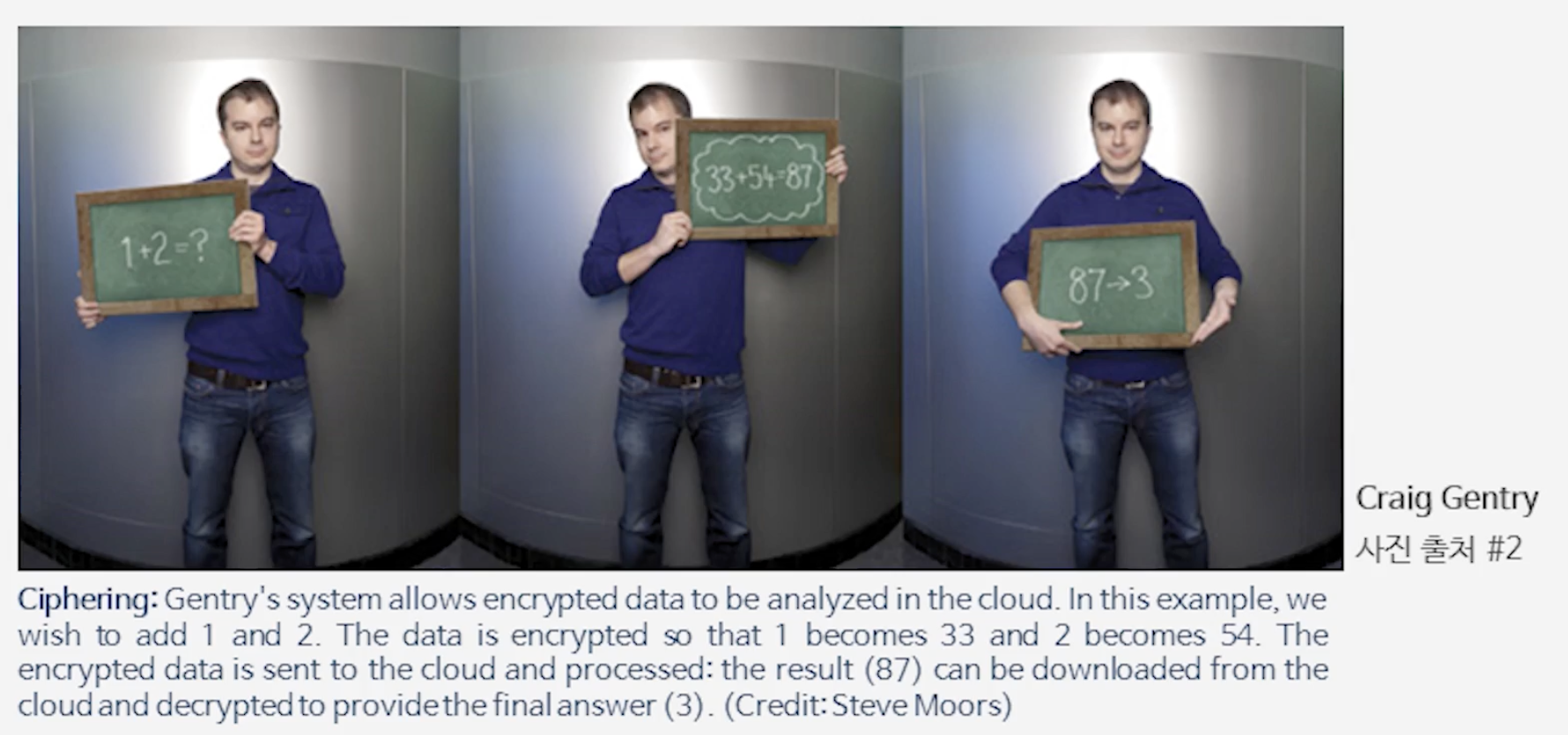
    예를 들어, 우리가 <strong>1 + 2</strong>라는 단순한 계산을 하고 싶다고 하자.  
    하지만 계산의 내용을 클라우드에 <em>노출하고 싶지 않다.</em>  
    이때 우리는 각 값을 암호화하여 클라우드에 보낸다.  
    예를 들어, <strong>1은 33</strong>, <strong>2는 54</strong>로 암호화된다.
  </p>

        <p>
    클라우드는 <strong>복호화 키를 전혀 알지 못한 채</strong>  
    단순히 암호문끼리의 덧셈(33 + 54)을 수행한다.  
    계산 결과로 얻은 <strong>87</strong>은 여전히 암호화된 상태이며,  
    우리는 이 값을 받아서 복호화하면 최종적으로 <strong>3</strong>을 얻는다.  
  </p>

        <p>
    이처럼 동형암호는 단순한 산술 연산뿐만 아니라  
    <strong>영상 처리나 머신러닝 모델 추론</strong>과 같은 복잡한 계산에도 확장될 수 있다.  
    예를 들어, 클라우드에게 두 장의 이미지를 암호화된 상태로 보내  
    “이 두 이미지가 같은지 비교해 달라”고 요청할 수 있다.  
    클라우드는 이미지 내용을 직접 보지 않고도 연산을 수행해  
    결과값만을 사용자에게 반환할 수 있다.
  </p>
      </div>
</details>

    <p align="center">
  <img src="/images/explorations/cheon/gentry-he.png" alt="Ciphering" style="max-width:100%; height:auto; display:block; margin:0 auto;" />
  <figcaption style="font-size:0.9em; color:gray; text-align:center;">
    [그림] 동형암호의 핵심 원리: 암호문 위에서의 연산
  </figcaption>
</p>

    <details style="margin-left:20px;">
  <summary>📘 <b>동형암호의 직관적 설명</b></summary>
  <div style="border:2px solid #007acc; border-radius:6px; padding:12px 15px; background:#f0f8ff; margin:12px 0; width:95%; font-size:0.95em;">
        <p>
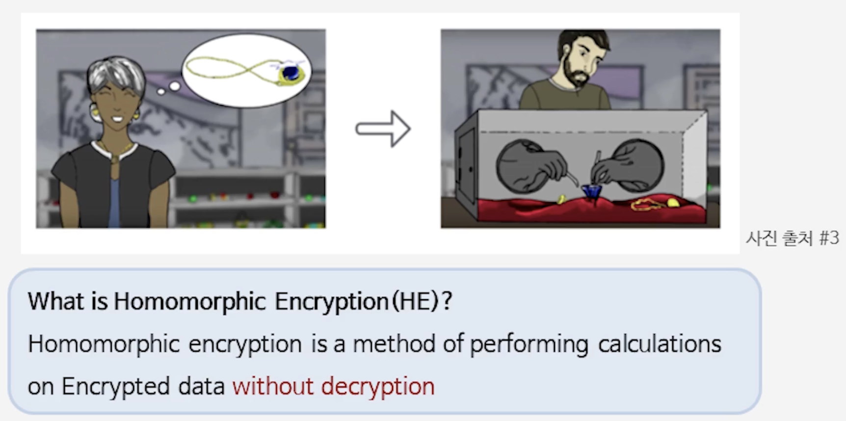
    간단한 비유로 설명하면, 전통적인 암호는 <strong>열쇠가 있어야만 여는 금고</strong>와 같습니다.  
    키가 없으면 그 안에 무엇이 있는지 전혀 알 수 없고, 아무런 조작도 할 수 없습니다.
  </p>

        <p>
    반면 동형암호는 <strong>“말랑말랑한 금고”</strong>와 비슷합니다. 금고 안의 내용(평문)은 외부에서 보이지 않지만,  
    외부에서 손(연산)을 넣어 내부의 값을 가공할 수 있습니다.  
    즉, 클라우드(연산자)는 복호화 키를 알지 못한 채도 암호문 위에서 덧셈·곱셈 같은 연산을 수행할 수 있고,  
    최종 결과는 여전히 암호화된 상태로 반환됩니다. 사용자는 그 결과를 복호화해 실제 정답을 얻습니다.
  </p>

        <p>
    예시: 의료 데이터의 경우, 환자의 원본 기록은 열리지 않은 상태로 보관됩니다.  
    연구자는 이 암호화된 데이터를 클라우드에 맡겨 통계분석이나 모델 추론을 수행하게 하고,  
    클라우드는 내용을 보지 못한 채 계산만 수행합니다. 계산 결과(예: 위험 지표)는 암호화된 상태로 돌아오고,  
    복호화 권한이 있는 사람만이 필요한 정보(예: 특정 진단의 유무 또는 요약된 수치)만 확인합니다.
  </p>

        <p>
    핵심은 <strong>"비밀은 지키면서도 필요한 계산은 수행할 수 있다"</strong>는 점입니다.  
    이 성질 덕분에 동형암호는 개인정보·의료·금융 데이터의 안전한 외부 계산(클라우드 기반 분석, 암호화된 ML 추론 등)에 유용합니다.
  </p>

      </div>
</details>

    <p align="center">
  <img src="/images/explorations/cheon/he-idea.png" alt="Ciphering" style="max-width:100%; height:auto; display:block; margin:0 auto;" />
  <figcaption style="font-size:0.9em; color:gray; text-align:center;">
    [그림] 동형암호의 핵심 아이디어: 보지 않고 계산하기
  </figcaption>
</p>

    <ul>
      <li>동형암호의 장·단점
        <ul>
          <li><strong>장점: 튜링완전성 (Turing-Complete)</strong>
            <ul>
              <li>암호화된 상태에서 <strong>AND, OR, NOT</strong> 연산이 모두 가능하다. 
즉, 컴퓨터가 수행할 수 있는 <strong>모든 연산 (검색·통계처리·머신러닝)</strong>을 암호화된 데이터 위에서 수행할 수 있다.<br />
→ 따라서 <strong>데이터 유출 위험을 원천 차단</strong>할 수 있다.</li>
            </ul>
          </li>
          <li><strong>단점</strong>
            <ul>
              <li><span style="color:red">암호문 크기 확장</span>: 평문 대비 <strong>약 $10$ ~ $100K$배</strong> (대칭키 방식은 약 $0.1$ ~ $1K$ 배 수준)</li>
              <li><span style="color:red">암·복호화 속도 저하</span>: AES ≈ $1 us$, RSA ≈ $1 ms$, HE ≈ <strong>수십 $ms$</strong></li>
              <li>암호문 연산 속도 저하: 특히 곱셈 연산은 평문 계산 대비 <strong>수백 배 이상 느림</strong></li>
              <li>응용별 성능 편차: 연산의 종류 (덧셈·곱셈·비교)에 따라 속도 차이가 크며, 효율을 높이기 위해 <strong>개별 최적화 알고리즘 및 구현 기술</strong>이 필요함
                <details style="margin-left:20px;">
  <summary>📘 예시 (복잡도 관점의 단순 모델) </summary>
  <div style="border:2px solid #007acc; border-radius:6px; padding:12px 15px; background:#f0f8ff; margin:12px 0; width:95%; font-size:0.95em;">

                    <p>
    - 128-bit 보안을 만족하기 위해 키 크기를 <strong>50배</strong> 늘린다고 가정하면,  
      계산량은 일반적으로 <code>O(n^2)</code> 복잡도를 가지므로  
      <strong>$50^2x = 2,500x$</strong> 배 증가하게 된다.  
  </p>

                    <p>
    - 그러나 <strong>빠른 곱셈 알고리즘</strong> (Fast Multiplication)을 적용하면  
      복잡도는 <code>O(nlog n)</code> 수준으로 개선되어  
      <strong>$(50 \log 50)x ≈ 2,000x$</strong> 배 정도로 줄어든다.  
  </p>

                    <p>
    👉 따라서, <strong>키 길이를 $50$배 늘려도 계산량은 약 $2,000$배 증가</strong>하게 된다.  
    즉, 보안 강도를 높이는 것은 필연적으로 연산 비용 증가를 수반한다.
  </p>

                    <p> 
    - 물론 위 계산은 <strong>최적화가 잘 이루어진 경우</strong>를 가정한 것이다.  
      실제로는 알고리즘과 구현 수준에 따라 성능 편차가 크며,  
      이러한 <strong>최적화(optimization)는 인공지능이 아니라 사람이 직접 설계</strong>해야 한다.  
      다시 말해, 알고리즘적·구현적 튜닝이 부족한 경우에는  
      여전히 <strong>수천 배에서 수만 배까지 느린 사례</strong>도 존재한다.
  </p>
                  </div>
</details>
              </li>
            </ul>
          </li>
        </ul>
      </li>
    </ul>

    <hr />

    <h3 id="section-1">2) 동형암호의 종류</h3>
    <ul>
      <li>
        <p><strong>정수 기반 동형암호 (Integer-based HE scheme)</strong> - <em>대칭키 방식</em> <br />
동형암호의 초기 형태는 <strong>정수 연산 기반</strong>으로 설계되었습니다. 대표적으로 RAD PH와 DGHV 스킴이 있습니다.</p>

        <ul>
          <li>RAD PH Scheme
            <ul>
              <li><strong>키 생성</strong>
                <ul>
                  <li>Secret Key: large prime $p$</li>
                  <li>Public Key: $n = p q_0$, $q$는 임의의 자연수</li>
                </ul>
              </li>
              <li><strong>암호화 (Encryption)</strong> : $Enc(m) = m + p q \pmod{n}$</li>
              <li><strong>복호화 (Decryption)</strong> : $Enc(m) \pmod p = m$ <br />
👉 Quadratic Complexity - O(λ²) in the bit-length of modulus n</li>
              <li><strong>덧셈 연산</strong><br />
\(Enc(m_1) + Enc(m_2) = (m_1 + p q_1) + (m_2 + p q_2)    
                    = (m_1 + m_2) + p(q_1 + q_2)
                    = Enc(m_1 + m_2)\)
👉 (m_1 + p의 배수) + (m_2 + p의 배수)로 생각하기!</li>
              <li><strong>곱셈 연산</strong><br />
\(Enc(m_1) * Enc(m_2) = (m_1 + p q_1) * (m_2 + p q_2)    
                    = (m_1 * m_2) + p(q_1 + q_2)
                    = Enc(m_1 * m_2)\)</li>
            </ul>
            <details style="margin-left:20px;">
  <summary>📘 결과: RAD PH의 장·단점 </summary>
  <div style="border:2px solid #007acc; border-radius:6px; padding:12px 15px; background:#f0f8ff; margin:12px 0; width:95%; font-size:0.95em;">

                <p>
    RAD PH는 구조가 단순하고 연산이 빠르며, 암호문 상태에서 덧셈·곱셈을 수행할 수 있다는 장점이 있다. 그러나 실전에서는 <strong>평문-암호문 쌍 공격</strong>과 <strong>곱셈 반복에 따른 잡음 누적</strong> 문제로 인해 그대로 사용하기엔 취약하다.
  </p>

                <p><strong>핵심 취약점</strong></p>
                <ul>
    <li><strong>평문-암호문 쌍에 취약:</strong> 암호문이 <code>m + p·q</code> 형태라 몇 개 쌍만 알면 <code>p</code>를 추정할 수 있다.</li>
    <li><strong>추측(guessing) 공격:</strong> 사람 문장은 패턴이 있어 일부만으로도 공격 실마리가 된다.</li>
    <li><strong>곱셈 반복 시 잡음 급증:</strong> 교차항과 <code>p^2</code> 항이 생겨 복호 실패 위험이 커진다.</li>
  </ul>

                <p>
  결론: <strong>효율 ↔ 안전성</strong>의 절충이 필요하다. Gentry의 부트스트래핑은 잡음을 관리해 반복 연산을 가능하게 했지만, 설계·파라미터·비용 문제가 남는다.   
  따라서 RAD PH 수준의 단순 정수 스킴은 "개념적으로는 멋지지만, 실제 보안 요구를 만족시키기엔 추가 보강이 필수"다.  
  </p>

              </div>
</details>
          </li>
          <li>DGHV HE scheme (on $\mathbb{Z}_{2}$)
            <ul>
              <li><strong>암호화</strong> : $Enc(m) = m + 2e + p q$
                <ul>
                  <li>$m \in {0,1}$: 메시지 비트</li>
                  <li>$e$: 작은 노이즈 (error term)</li>
                  <li>$p, q$: 큰 정수</li>
                  <li><strong>핵심 아이디어</strong><br />
DGHV는 RAD PH와 달리 암호문에 <strong>작은 노이즈 $e$</strong>를 추가한다. <br />
따라서 공격자가 평문을 어느 정도 추측하더라도, 노이즈까지 함께 복원하지 못하면 암호문 구조를 직접 이용한 공격이 어려워진다.</li>
                </ul>
              </li>
              <li>
                <p><strong>동형성</strong><br />
DGHV 역시 암호문 상태에서 <strong>덧셈과 곱셈</strong>을 지원한다. <br />
따라서 복호화 결과는 각각 평문의 덧셈 및 곱셈에 대응한다.</p>
              </li>
              <li>
                <p><strong>한계</strong><br />
문제는 연산, 특히 <strong>곱셈을 반복할수록 노이즈가 증가한다</strong>는 점이다. <br />
노이즈가 일정 수준을 넘으면 복호화가 실패하므로, 초기 스킴은 계산 가능한 깊이(multiplicative depth)가 제한된다.</p>
              </li>
              <li>
                <p><strong>암호문 크기가 커지는 이유</strong><br />
여러 번의 곱셈을 지원하려면 중간 계산 과정에서 증가하는 노이즈와 비트 길이를 감당할 <strong>여유 공간</strong>이 필요하다.<br />
이 때문에 동형암호는 일반 암호보다 훨씬 큰 암호문 크기를 갖게 된다.</p>
              </li>
              <li><strong>특징</strong>
                <ul>
                  <li><span style="color:red"><strong>양자 컴퓨팅에 대해 안전 (Post-Quantum Secure)</strong></span></li>
                  <li>정수 기반 대신 <strong>다항식 링</strong> 구조를 사용하는 고도화된 확장 버전 존재: <br />
$R_q = \mathbb{Z}_q[x] / (x^n + 1)$</li>
                </ul>
              </li>
              <li>✅ <strong>의의:</strong><br />
DGHV는 <em>Craig Gentry의 Fully Homomorphic Encryption (FHE)</em>의 초기 형태로, “잡음을 제어하며 연산을 확장하는” 아이디어의 기반이 되었다.</li>
            </ul>

            <details style="margin-left:20px;">
  <summary>📘 왜 DGHV가 RAD PH보다 더 안전한가?</summary>
  <div style="border:2px solid #007acc; border-radius:6px; padding:12px 15px; background:#f0f8ff; margin:12px 0; width:95%; font-size:0.95em;">

                <p>DGHV에서는 암호문이 $m + 2e + pq$ 형태이므로, 공격자는 평문 $m$뿐 아니라 작은 노이즈 $e$까지 함께 고려해야 한다. 따라서 RAD PH처럼 단순한 평문-암호문 대응만으로 secret structure를 추정하기가 훨씬 어려워진다.</p>

                <p>이 계열의 안전성은 <strong>Approximate GCD 문제</strong>와 관련되며, 이후 격자 기반 난제와의 연결성도 연구되었다.</p>

              </div>
</details>

            <details style="margin-left:20px;">
  <summary>📘 noise와 bootstrapping의 의미</summary>
  <div style="border:2px solid #007acc; border-radius:6px; padding:12px 15px; background:#f0f8ff; margin:12px 0; width:95%; font-size:0.95em;">

                <p>DGHV에서 가장 큰 제약은 <strong>곱셈이 반복될수록 노이즈가 커진다</strong>는 점이다.<br />
  따라서 암호문은 처음부터 어느 정도의 계산 여유를 갖도록 크게 설계되어야 한다.</p>

                <p>하지만 계산 깊이가 계속 증가하면 결국 복호화가 불가능해진다.<br />
  Gentry의 핵심 아이디어는 이 한계를 넘기 위해, <strong>복호화 회로 자체를 암호문 위에서 다시 평가하여 노이즈를 줄이는 bootstrapping</strong>을 수행하는 것이었다.</p>

                <p>즉, bootstrapping은 암호화된 상태를 “다시 사용 가능한 상태”로 정리해 주는 과정이라고 볼 수 있다.</p>

              </div>
</details>
          </li>
        </ul>
      </li>
    </ul>

  </div>
</details>]]></content><author><name>Jihyung Kook (국지형)</name><email>jhkook30@gmail.com</email></author><category term="cryptography" /><category term="homomorphic-encryption" /><category term="lattice-based-cryptography" /><summary type="html"><![CDATA[해당 포스트는 서울대학교 천정희 교수님의 암호론 강의를 기반으로 작성하였다. 이번 포스트에서는 ‘동형암호의 개요’에 대한 내용을 요약•정리하고자 한다.]]></summary></entry><entry><title type="html">Post-Quantum Cryptography</title><link href="https://jhkook30.github.io/posts/2025/09/crypto-note-3/" rel="alternate" type="text/html" title="Post-Quantum Cryptography" /><published>2025-09-17T00:00:00+09:00</published><updated>2025-09-17T00:00:00+09:00</updated><id>https://jhkook30.github.io/posts/2025/09/crypto-note-3</id><content type="html" xml:base="https://jhkook30.github.io/posts/2025/09/crypto-note-3/"><![CDATA[<!-- 배너 이미지 + 링크 -->
<p><a href="https://etl.snu.ac.kr/courses/67ac1cbf62137e66b0296b17" target="_blank">
  <img src="/images/explorations/cheon/crypto-cheon.png" alt="서울대학교 천정희 교수님의 암호론 강의" style="width:100%; border-radius:10px; margin-bottom:20px;" />
</a></p>

<p>해당 포스트는 <em>서울대학교 천정희 교수님의 암호론 강의</em>를 기반으로 작성하였다. 이번 포스트에서는 <strong>‘양자내성암호’</strong>에 대한 내용을 요약•정리하고자 한다.</p>

<!--more-->

<details>
  <summary>
  <span style="font-size:1.25em; font-weight:bold;">
    1. 양자내성(Quantum-resistant) 공개키암호
  </span>
  </summary>
  <div>

    <hr />

    <h3 id="section">1) 양자 컴퓨터의 전망</h3>
    <ul>
      <li>약 15년 이내에 기존 암호를 공격할 수준의 양자 컴퓨터 도래 예상
        <details style="margin-left:20px;">
  <summary>📘 양자컴퓨터, 정말 만들 수 있을까?</summary>
  <div style="border:2px solid #007acc; border-radius:6px; padding:12px 15px; background:#f0f8ff; margin:12px 0; width:95%; font-size:0.95em;">

            <p><strong>양자컴퓨터, 아직은 Open Problem</strong></p>
            <ul>
              <li>양자컴퓨터를 <strong>충분히 큰 규모로 만들 수 있느냐</strong>는 아직도 <em>open problem</em>이다.</li>
              <li>현재 우리는 소규모의 <strong>양자 비트(Qubit)</strong>를 다루는 장치는 만들었지만, 이를 <strong>scalable</strong>하게 확장할 수 있을지는 불확실하다.</li>
              <li>양자컴퓨터는 0과 1을 동시에 다루지만, 이로 인해 잡음(noise)와 decoherence가 심각해지고, <strong>여러 큐비트를 동시에 안정적으로 제어하는 것</strong>이 매우 어렵다.</li>
              <li>그래서, 예를 들어 1,000큐비트로 확장하게 되면 <strong>오류(Error)</strong>가 너무 커진다.</li>
            </ul>

            <hr />

            <p><strong>양자컴퓨터의 두 가지 구현 방식</strong></p>
            <ul>
              <li><strong>Quantum Gate 방식</strong>: 전통적으로 암호학에 위협적인 방식이지만, 현재 발전 속도는 더딘 편이다.</li>
              <li><strong>Quantum Annealing(어닐링) 방식</strong>: D-Wave, Google 등에서 이미 수백 큐비트까지 구현했으나, 이 방식은 <strong>암호를 다항식 시간 내에 깨지는 못한다.</strong><br />
대신, <strong>검색·최적화 문제를 빠르게 푸는 데 유용</strong>하며, 실제로 산업 응용에서 활발히 연구 중이다.</li>
              <li>따라서, 암호를 직접적으로 해독할 수 있는 게이트 기반 양자컴퓨터가 언제 등장할지는 불확실하다.<br />
어떤 전문가는 <strong>15년</strong>, 또 어떤 전문가는 <strong>150년</strong>을 예상할 정도로 의견 차이가 크다.</li>
            </ul>

          </div>
</details>
      </li>
      <li>현재 널리 쓰이는 모든 공개키 암호(ECC/RSA 등)은 Shor’s Algorithm 때문에 공격 가능
        <details style="margin-left:20px;">
  <summary>📘 Shor's Algorithm 자세히 보기</summary>
  <div style="border:2px solid #007acc; border-radius:6px; padding:12px 15px; background:#f0f8ff; margin:12px 0; width:95%; font-size:0.95em;">

            <ul>
              <li>Shor의 알고리즘은 인수분해와 이산로그 문제의 복잡도를 <strong>지수적(exponential)</strong>에서 <strong>다항식(polynomial)</strong> 수준으로 낮춘다.</li>
              <li>따라서 현재 우리가 사용하는 RSA, ECC 같은 공개키 암호는 양자컴퓨터에서 효율적으로 깨질 수 있다.</li>
              <li>예: 약 <strong>1,000 큐비트</strong> 정도의 양자컴퓨터가 현실화되면 RSA-2048 수준의 암호도 짧은 시간 안에 풀릴 수 있다고 예측한다.</li>
            </ul>

          </div>
</details>
      </li>
      <li>반면, 대칭키 암호/해쉬 함수는 키의 길이, 해쉬의 길이를 두 배로 늘리면 기존 수준의 보안성 유지 가능</li>
    </ul>

    <hr />

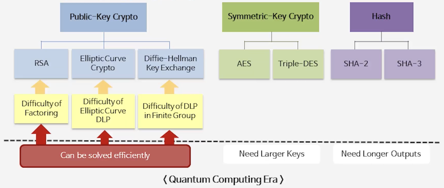
    <h3 id="contemporary-cryptography">2) Contemporary Cryptography</h3>
    <p align="center">
  <img src="/images/explorations/cheon/contemporary-cryptography.png" alt="Contemporary Cryptography" style="max-width:100%; height:auto; display:block; margin:0 auto;" />
  <figcaption style="font-size:0.9em; color:gray; text-align:center;">
    [그림] 양자 컴퓨터 시대의 암호학적 영향
  </figcaption>
</p>

    <ul>
      <li>공개키 암호 (RSA, ECC, DH): Shor 알고리즘 때문에 안전하지 않음 → 비트 수 늘려도 소용 없음</li>
      <li>대칭키 암호 (AES 등): 키 길이를 2배로 늘리면 안전성 유지 가능 (예: AES-256 권장)</li>
      <li>
        <p>해시 함수 (SHA 계열): 출력 길이를 3배로 늘려야 같은 수준의 보안성 유지 가능</p>
      </li>
      <li><strong>요약: 누가 무엇에 영향주는가</strong>
        <ul>
          <li><strong>Shor’s algorithm</strong>: 공개키 암호(인수분해·이산로그 기반)를 양자환경에서 <strong>다항식 시간(polynomial time)</strong> 내에 풀어버리는 알고리즘 → 공개키 계열은 근본적 위협</li>
          <li><strong>Grover’s algorithm</strong>: 대칭키/해시의 무차별 공격을 <strong>제곱근(quadratic)</strong> 속도로 가속화하는 알고리즘 → 완전 붕괴는 아니며, 키/출력 길이를 늘려 방어 가능</li>
        </ul>

        <details style="margin-left:20px;">
  <summary>📘 왜 이렇게 되는 걸까?</summary>
  <div style="border:2px solid #007acc; border-radius:6px; padding:12px 15px; background:#f0f8ff; margin:12px 0; width:100%; font-size:0.95em;">
            <ul>
              <li><strong>공개키 (Shor)</strong>
                <ul>
                  <li>고전적 최선: 인수분해·이산로그는 지수 시간(대략 $(2^{n})$ 또는 유사) 소모</li>
                  <li>Shor: 이를 <strong>다항식 시간(예: poly($n$))</strong>으로 해결 → 비트 길이 확대만으로는 방어 불가</li>
                </ul>
              </li>
              <li><strong>대칭키 (Grover)</strong>
                <ul>
                  <li>고전적 무차별 검색: $O(2^{n})$ (키 길이: $n$)</li>
                  <li>Grover: $O(2^{\frac{n}{2}})$으로 가속 — 즉 <strong>제곱근(Quadratic) 속도 향상</strong></li>
                  <li>결과: 키 길이를 <strong>2배</strong> 하면 기존 수준의 보안 유지 가능 (예: AES-128 → AES-256 권장)</li>
                </ul>
              </li>
              <li><strong>해시(충돌/프리이미지)</strong>
                <ul>
                  <li>고전적 충돌 저항: $2^{\frac{n}{2}}$ (출력 길이: $n$)</li>
                  <li>양자 영향 하의 충돌/프리이미지 복잡도는 알고리즘과 공격 모델에 따라 달라지지만, 실무에서는 <strong>출력 길이를 충분히 늘림(권장: 약 3배 규칙)</strong>으로 안전성을 확보하는 관점이 사용</li>
                  <li>따라서 “128비트 수준의 안전성”을 목표로 하면 <strong>출력 길이를 256비트가 아니라 더 늘려(약 384비트 권장)</strong>야 한다는 주장으로 정리되는 경우가 있음</li>
                </ul>
              </li>
            </ul>

          </div>
</details>
      </li>
    </ul>

    <hr />

    <h3 id="post-quantum-cryptography-1">3) Post-Quantum Cryptography (1)</h3>
    <ul>
      <li><strong>2016년</strong>, 미국 국가안보국(NSA)은 <em>“머지않은 미래(not too distant future)에 Post-Quantum Cryptography (PQC)로 전환하겠다”</em>고 발표</li>
      <li>곧바로 미국 국립표준기술연구소(NIST)가 <strong>PQC 표준화 프로젝트</strong>를 시작하면서 오늘날의 Kyber, Dilithium 등 PQC 알고리즘 경쟁이 본격화
        <ul>
          <li>목표: Post-Quantum 공개키 암호(Encryption / Signature / Key Exchange)의 표준화</li>
        </ul>

        <details style="margin-left:20px;">
  <summary>📘 당시 상황을 조금 더 살펴보기</summary>
  <div style="border:2px solid #007acc; border-radius:6px; padding:12px 15px; background:#f0f8ff; margin:12px 0; width:100%; font-size:0.95em;">

            <ul>
              <li>당시 미국 정부는 <strong>Suite A/B 암호 체계</strong>를 따랐는데, Suite B에는 <strong>AES</strong>와 <strong>ECC</strong>를 포함한다</li>
              <li>즉, 미국과 외국 정부가 안전하게 통신하려면 ECC 지원이 필수였다.</li>
              <li>그런데 NSA가 ECC 도입을 중단하고 PQC로 전환하겠다고 선언하면서, 사실상 <strong>전 세계가 따라야 하는 신호</strong>가 되었다.</li>
              <li>NSA 발표 직후, NIST는 <strong>2016년 가을 Call for Proposals</strong>, <strong>2017년 Submission 마감</strong> 일정을 공개하며 PQC 표준화 작업에 착수했다.</li>
            </ul>

          </div>
</details>
      </li>
    </ul>

    <hr />

    <h3 id="post-quantum-cryptography-2">4) Post-Quantum Cryptography (2)</h3>
    <ul>
      <li>양자내성암호의 전제 조건
        <ul>
          <li>가설 1. $P ≠ NP$<br />
→ 양자컴퓨터가 등장해도 $NP$ 문제 전체를 쉽게 풀 수 있다는 근거는 없다.</li>
          <li>가설 2. NP-hard 기반 안전성<br />
→ 암호는 보통 NP-hard 문제와 동치가 아니라, 그 위에 기반한다고 본다.</li>
        </ul>

        <details style="margin-left:20px;">
  <summary>📘 더 자세히 보기</summary>
  <div style="border:2px solid #007acc; border-radius:6px; padding:12px 15px; background:#f0f8ff; margin:12px 0; font-size:0.95em;">
            <ul>
              <li>가설 1 (P ≠ NP)
                <ul>
                  <li>퀀텀 알고리즘은 병렬화와 유사한 성질을 보이지만, NP 문제 전체를 풀 수 있다는 증거는 없다.</li>
                  <li>따라서 P와 NP의 분리는 유지된다고 보는 것이 일반적이다.</li>
                </ul>
              </li>
              <li>가설 2 (기반 vs. 동치)
                <ul>
                  <li>암호 설계에서 특정 NP-hard 문제와 정확히 동치임을 보장할 수는 없다.</li>
                  <li>하지만 “그 문제를 기반으로 한다(based on)” 정도면 연구자 사회에서 충분히 인정한다.</li>
                  <li>예: RSA는 인수분해와 동치는 아니지만, 인수분해 문제에 기반해 안전성을 설명한다.</li>
                </ul>
              </li>
            </ul>
          </div>
</details>
      </li>
    </ul>

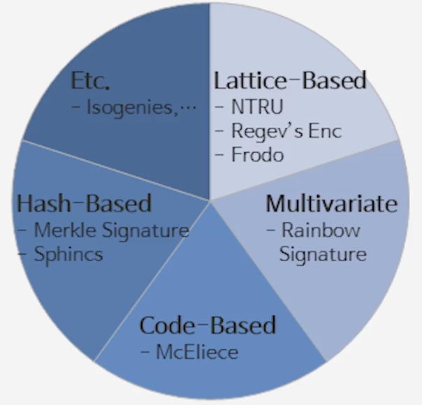
    <p align="center">
  <img src="/images/explorations/cheon/pqc-family.png" alt="PQC Family" style="max-width:40%; height:auto; display:block; margin:0 auto;" />
  <figcaption style="font-size:0.9em; color:gray; text-align:center;">
    [그림] 양자내성암호의 대표적 암호 계열
  </figcaption>
</p>

    <ul>
      <li><span style="color:red">Lattice-based가 주목받는 이유</span>
        <ul>
          <li><strong>보안성</strong>: 난이도가 높은 <em>격자 문제(lattice problems)</em> 에 기반 (NP-hard)</li>
          <li><strong>효율성</strong>: 구현이 빠르고, 실제 하드웨어/소프트웨어에 적합</li>
          <li><strong>범용성</strong>: 동형암호(HE), 신원기반암호(IBE) 등 다양한 응용 가능
            <ul>
              <li>동형암호(HE): 암호화된 상태에서 연산을 직접 수행할 수 있는 암호</li>
              <li>신원기반암호(IBE): 이메일 주소 같은 신원 자체를 공개키로 삼는 암호</li>
            </ul>
          </li>
        </ul>
      </li>
    </ul>

    <hr />

    <h3 id="light-weight-">5) 경량 (Light Weight) 공개키암호</h3>
    <ul>
      <li>기존 공개키 암호의 기반 난제: 지수승 연산 (예. RSA, ECC → $a \mapsto a^b$)
        <ul>
          <li>지수 연산은 본질적으로 계산량이 크고, 효율성에도 한계가 있음</li>
        </ul>
      </li>
      <li>그렇다면, <strong>“지수승 대신 곱셈만으로도 안전한 암호를 만들 수 없을까?”</strong>란 질문이 나옴
        <ul>
          <li>곱셈은 지수승보다 계산이 훨씬 빠르지만 (제곱 정도의 계산량),<br />
$a \mapsto ab$는 너무 단순해서 일방향 함수로 쓰기에는 안전성 부족</li>
        </ul>
      </li>
    </ul>

    <details style="margin-left:20px;">
  <summary><b><span style="color:red">📘 Lattice 접근법</span></b></summary>
  <div style="border:2px solid #007acc; border-radius:6px; padding:12px 15px; background:#f0f8ff; margin:12px 0; width:100%; font-size:0.95em;">

        <ul>
          <li>격자 기반 암호는 단순 곱셈 $ab$에 <strong>노이즈(잡음)</strong>를 더해서 문제를 어렵게 만든다.
            <ul>
              <li>$a \mapsto ab + \text{noise}$ 형태</li>
              <li>계산량은 <em>quadratic</em> 수준을 유지하면서도, 노이즈 때문에 문제는 어렵게 정의된다.</li>
              <li>노이즈가 들어가면 단일 해답이 아니라 <strong>많은 경우의 수(case)</strong>가 생겨서 공격이 어렵다.</li>
            </ul>

            <p>→ 이런 성질 덕분에 Lattice 기반 암호는 <span style="color:red"><em>효율성(빠름)과 안전성(어려움)</em></span> 을 동시에 노릴 수 있다.</p>
          </li>
        </ul>

      </div>
</details>

  </div>
</details>

<hr />

<details>
  <summary>
  <span style="font-size:1.25em; font-weight:bold;">
    2. 격자기반 양자내성암호
  </span>
  </summary>
  <div>

    <hr />

    <h3 id="geometry-of-numbers-lattices-1">1) Geometry of Numbers: Lattices (1)</h3>
    <ul>
      <li>격자란 무엇인가?
        <ul>
          <li>격자(Lattice)는 $\mathbb{R}^n$ 안에 있는 <u>이산적인(discrete)</u> 점들의 집합
            <ul>
              <li>이산적이란? 임의의 격자점에서 작은 원을 그리면, 그 안에는 자기 자신만 있고 다른 격자점은 들어오지 않는다.</li>
            </ul>
          </li>
          <li>일차독립 벡터 $v_1, \dots, v_m \in \mathbb{R}^n$이 주어지면,
\(L = \mathbb{Z}v_1 + \cdots + \mathbb{Z}v_m\) 
(선형결합)로 정의</li>
        </ul>

        <details style="margin-left:20px;">
  <summary><b>📘 기저 (Basis)와 기저 행렬</b></summary>
  <div style="border:2px solid #007acc; border-radius:6px; padding:12px 15px; background:#f0f8ff; margin:12px 0; width:100%; font-size:0.95em;">
            <ul>
              <li><strong>기저 (Basis)</strong>
                <ul>
                  <li>$v_1, \dots, v_m$을 격자의 <strong>기저(basis)</strong>라고 한다.</li>
                  <li>이 기저 벡터들을 <strong>정수배</strong>해서 나오는 모든 점들이 격자점이다.</li>
                  <li>벡터공간의 기저와 비슷하지만, 차이가 있다 → 벡터공간은 실수배/유리수배를 허용하지만, 격자는 정수배만 허용한다.</li>
                </ul>
              </li>
              <li><strong>기저 행렬 (Basis Matrix)</strong>
                <ul>
                  <li>기저 벡터들을 모아 $B = [v_1 ; v_2 ; \cdots ; v_m]$라고 하면,<br />
모든 격자점 $v$는 \(v = Bx, \quad x \in \mathbb{Z}^m\) 형태로 쓸 수 있다.</li>
                </ul>
              </li>
            </ul>
          </div>
</details>

        <details style="margin-left:20px;">
  <summary><b>📘 격자의 부피 (Determinant)</b></summary>
  <div style="border:2px solid #007acc; border-radius:6px; padding:12px 15px; background:#f0f8ff; margin:12px 0; width:100%; font-size:0.95em;">
            <ul>
              <li><strong>격자의 부피(Det(L))</strong>는 기저 벡터들이 만드는 평행다면체(parallelepiped)의 부피와 같다.</li>
              <li>\(\det(L) = \det[v_1 ; v_2 ; \cdots ; v_m]\)
로 정의된다.</li>
              <li>💡 직관적으로, 2차원 (평행사변형의 넓이), 3차원 (평행육면체의 부피), 4차원 이상 (일반화된 평행다면체의 부피)</li>
              <li>단, 정사각행렬이 아닐때는?
                <ul>
                  <li>예: 3차원 공간에 벡터가 두 개만 있으면 3×2 행렬 → 정사각형 아님</li>
                  <li>이 경우, 두 벡터가 span하는 2차원 평면 위에서 생각한다.</li>
                  <li>즉, 그 평면 안에서 2×2 행렬로 다시 보고, 그 평행사변형의 넓이로 정의할 수 있다.</li>
                </ul>
              </li>
            </ul>
          </div>
</details>

        <details style="margin-left:20px;">
  <summary><b>📘 정수론과 격자의 연결</b></summary>
  <div style="border:2px solid #007acc; border-radius:6px; padding:12px 15px; background:#f0f8ff; margin:12px 0; width:100%; font-size:0.95em;">
            <ul>
              <li>정수론에는 원래 거리 개념이 없다.<br />
→ 예: 모듈러 $p$에서 2와 5 중 어느 쪽이 더 크다고 말할 수 없다.</li>
              <li>하지만 격자를 도입하면 거리 개념을 가져올 수 있고, 덕분에 “가장 작은 해(솔루션)” 같은 문제를 논할 수 있다.
                <ul>
                  <li>응용 예시: Four Square Theorem <br />
→ 모든 자연수는 네 제곱수의 합으로 쓸 수 있다 <br />
     \(n = a^2 + b^2 + c^2 + d^2\)</li>
                </ul>
              </li>
            </ul>

          </div>
</details>
      </li>
      <li>격자와 벡터공간의 차이
        <ul>
          <li>벡터공간에서는 실수( $\mathbb{R}$ )나 유리수( $\mathbb{Q}$ ) 배수가 허용<br />
→	예: 벡터를 $0.1$배, $1.5$배 등으로도 만들 수 있음</li>
          <li>격자에서는 정수($\mathbb{Z}$) 배수만 허용<br />
→	예: 벡터를 $1$배, $2$배, $-3$배 하는 식<br />
  $\therefore$ 격자는 벡터공간의 “부분집합”이지만, 모든 점이 격자점인 것은 아니다.</li>
        </ul>
      </li>
      <li>격자의 어려운 문제들
        <ul>
          <li><strong>Shortest Vector Problem (SVP)</strong>: 0이 아닌 가장 짧은 벡터를 찾는 문제 (어렵다).</li>
          <li><strong>Closest Vector Problem (CVP)</strong>: 임의의 점이 주어졌을 때 가장 가까운 격자점을 찾는 문제 (역시 어렵다).</li>
          <li>이 난제들이 바로 <strong>격자 기반 암호의 안전성</strong>을 뒷받침한다.</li>
        </ul>
      </li>
    </ul>

    <hr />

    <h3 id="geometry-of-numbers-lattices-2">2) Geometry of Numbers: Lattices (2)</h3>

    <ul>
      <li>Shortest Vector Problem (SVP):<br />
격자 $L$이 주어졌을 때, 0이 아닌 벡터 중에서 가장 짧은 벡터를 찾으시오.</li>
    </ul>

    <p align="center">
  <img src="/images/explorations/cheon/lattice-svp.png" alt="Lattice SVP" style="max-width:80%; height:auto; display:block; margin:0 auto;" />
  <figcaption style="font-size:0.9em; color:gray; text-align:center;">
    [그림] Shortest Vector Problem
  </figcaption>
</p>

    <details style="margin-left:20px;">
  <summary><b>📘 어떤 경우에 어려울까?</b></summary>
  <div style="border:2px solid #007acc; border-radius:6px; padding:12px 15px; background:#f0f8ff; margin:12px 0; width:100%; font-size:0.95em;">

        <ul>
          <li><strong>직교 기저(orthogonal basis)</strong>일 때는 쉽다.
            <ul>
              <li>기저 벡터들이 서로 수직이라면, 임의의 점에서 <strong>정사영(projection)</strong>을 이용해 쉽게 가까운 격자점이나 최소 벡터를 찾을 수 있다.</li>
              <li>예: (–1, 0)이나 (0, –2) 같은 경우 → 바로 확인 가능.</li>
            </ul>
          </li>
          <li><strong>기저가 “누워 있는 경우(직교가 아닌 경우)”</strong>에는 어렵다.
            <ul>
              <li>기저 벡터들이 수직에서 멀어질수록, 한 점에 대해 가까운 후보 격자점이 여러 개 생긴다.</li>
              <li>정사영 방식이 통하지 않아, 최소 벡터를 찾는 일이 훨씬 복잡해진다.</li>
              <li>예: (–5, –1)과 (11, 3) 같은 벡터 → 어느 게 shortest인지 직관적으로 알기 어려움.</li>
            </ul>
          </li>
          <li>이 때문에 <strong>직교 기저</strong>가 중요하다.<br />
<span style="color:red">실제로 격자 기저를 “직교에 가깝게” 바꿔주는 방법으로 <strong>Gram–Schmidt 정규화</strong> 같은 기법이 중요하게 쓰인다.</span></li>
        </ul>

      </div>
</details>

    <details style="margin-left:20px;">
  <summary><b>📘 기저를 좋게 만드는 과정</b></summary>
  <div style="border:2px solid #007acc; border-radius:6px; padding:12px 15px; background:#f0f8ff; margin:12px 0; width:100%; font-size:0.95em;">

        <p><strong>👉 Gram–Schmidt 정규화 (실수배 허용)</strong></p>
        <ul>
          <li>주어진 기저 벡터들을 <strong>서로 직교하는 기저</strong>로 바꿔주는 방법</li>
          <li>벡터 $v_2$에서 $v_1$ 방향 성분을 빼주면, $v_1$과 직교하는 새로운 벡터가 된다.</li>
          <li>이런 식으로 순차적으로 직교 성분을 제거하면, 원래와 같은 공간을 span하는 <strong>직교 기저</strong>를 얻을 수 있다.</li>
          <li>
            <p>단점: 격자는 <strong>정수배만 허용</strong>하는데, Gram–Schmidt는 실수배를 쓰므로 격자 안에서는 바로 적용 불가.</p>
          </li>
          <li>Gram–Schmidt 정규화 (Step-by-Step)</li>
        </ul>

        <table>
    <tr>
      <td align="center">
        <img src="/images/explorations/cheon/gram/gram_schmidt_step1_v2.png" alt="Step 1" width="200" /><br />
        <sub>Step 1 — 원래 기저 \(v_1, v_2\)</sub>
      </td>
      <td align="center">
        <img src="/images/explorations/cheon/gram/gram_schmidt_step2_v2.png" alt="Step 2" width="200" /><br />
        <sub>Step 2 — \(v_2\)를 \(v_1\) 위로 정사영</sub>
      </td>
    </tr>
  </table>

        <table>
    <tr>
      <td align="center">
        <img src="/images/explorations/cheon/gram/gram_schmidt_step3_v2.png" alt="Step 3" width="200" /><br />
        <sub>Step 3 — \(u_2 = v_2 - \mathrm{proj}_{v_1}(v_2)\)</sub>
      </td>
      <td align="center">
        <img src="/images/explorations/cheon/gram/gram_schmidt_step4_v2.png" alt="Step 4" width="200" /><br />
        <sub>Step 4 — 직교 기저 \(\{u_1, u_2\}\)</sub>
      </td>
    </tr>
  </table>

        <hr />

        <p><strong>👉 가우스 환원 (정수배만 허용)</strong></p>
        <ul>
          <li>격자 기저를 <strong>더 수직에 가깝게</strong> 만드는 방법.</li>
          <li>$v_2$에서 $v_1$의 정수배를 반복해서 빼주면, 점점 짧고 수직에 가까운 벡터가 만들어진다.</li>
          <li>이 과정을 번갈아 적용하면, 결국 “더 좋은 기저”를 찾을 수 있다.</li>
          <li>가우스는 2차원에서 이 환원이 항상 <strong>유한 번 안에 끝난다</strong>는 것을 증명했다.</li>
        </ul>

        <p align="center">
    <img src="/images/explorations/cheon/gram/gauss_reduction.png" alt="Gauss Reduction Steps" style="max-width:100%; height:auto; display:block; margin:0 auto;" />
    <figcaption style="font-size:0.9em; color:gray; text-align:center;">
      [그림] Gauss Reduction Steps
    </figcaption>
  </p>

        <hr />

        <p><strong>👉 차원 확장과 난이도</strong></p>
        <ul>
          <li>3차원, 4차원에서도 비슷한 아이디어로 기저를 개선할 수 있다.</li>
          <li>하지만 차원이 커질수록 계산량이 <strong>기하급수적으로 증가</strong>한다.</li>
          <li>결국 <strong>고차원 격자에서 SVP를 푸는 문제는 NP-hard</strong>임이 1997년에 증명되었다.</li>
        </ul>

      </div>
</details>

    <hr />

    <h3 id="geometry-of-numbers-lattices-3">3) Geometry of Numbers: Lattices (3)</h3>
    <ul>
      <li>Hardness of SVP
        <ul>
          <li>SVP는 NP-hard로 알려져 있음 → 고차원 격자에서는 효율적 해법 없음</li>
          <li>하지만 수학자들은 “격자점의 최소 길이 벡터는 어느 정도일까?”라는 질문을 오래 연구함</li>
        </ul>

        <details style="margin-left:20px;">
  <summary><b>📘 Minkowski의 통찰</b></summary>
  <div style="border:2px solid #007acc; border-radius:6px; padding:12px 15px; background:#f0f8ff; margin:12px 0; width:100%; font-size:0.95em;">

            <ul>
              <li><strong>격자의 볼륨 (Det)</strong>
                <ul>
                  <li>기저 벡터들이 만드는 평행사변형/평행육면체의 부피는 격자에 대한 <strong>불변량</strong>이다.</li>
                  <li>기저를 $v_1, v_2$로 잡든, $v_2, v_3$로 잡든 $\det(L)$ 값은 변하지 않는다.</li>
                </ul>
              </li>
              <li><strong>직교 기저로 생각해보기</strong>
                <ul>
                  <li>만약 $n$차원에서 모든 기저 벡터가 <strong>서로 직교</strong>하고, 길이가 모두 $\ell$이라면,<br />
\(\det(L) = \ell^n \;\;\Rightarrow\;\; \ell = \det(L)^{1/n}\)</li>
                  <li>따라서 최소 벡터의 길이는<br />
\(\lambda_1(L) \leq \det(L)^{1/n}\)<br />
정도일 것이라 직관할 수 있다.</li>
                </ul>
              </li>
              <li><strong>Minkowski의 정리</strong>
                <ul>
                  <li>실제 일반 격자에서는 기저가 직교하지 않으므로, 위 직관보다 더 넉넉한 상한이 필요하다.</li>
                  <li>Minkowski는 다음을 증명했다:<br />
\(\lambda_1(L) \leq \sqrt{n}\,\det(L)^{1/n}\)</li>
                  <li>즉, 최소 벡터의 길이는 <strong>격자의 부피(det)와 차원(n)에 의해 제약</strong>된다.</li>
                  <li>고차원에서는 $\sqrt{n}$보다 더 좋은 값이 알려진 경우도 있지만, $n \geq 10$ 이상에서는 여전히 정확한 상한이 미해결 문제다.</li>
                </ul>
              </li>
            </ul>

          </div>
</details>
      </li>
      <li>수학 문제를 다루는 세 가지 질문
        <ol>
          <li>Existence (존재성): 해가 존재하는가?</li>
          <li>Uniqueness / Number (유일성·개수): 하나인가, 여러 개인가?</li>
          <li>Computability (계산 가능성): 실제로 계산 가능한가?</li>
        </ol>
      </li>
    </ul>

    <details style="margin-left:20px;">
  <summary><b>📘 LLL 알고리즘</b></summary>
  <div style="border:2px solid #007acc; border-radius:6px; padding:12px 15px; background:#f0f8ff; margin:12px 0; width:100%; font-size:0.95em;">

        <ul>
          <li><strong>배경</strong>
            <ul>
              <li>Shortest Vector Problem (SVP)는 NP-hard → “계산 가능성”에 대한 해답이 필요하다.</li>
            </ul>
          </li>
          <li><strong>아이디어</strong>
            <ul>
              <li>짧은 벡터를 찾으려면 더 좋은 기저(직교에 가까운 기저)가 필요하다.</li>
              <li>Gram–Schmidt 정규화는 실수 계수를 사용해야 해서 정수 격자에는 그대로 적용 불가</li>
              <li>LLL(1982)은 <strong>Gram–Schmidt를 기반</strong>으로 하되, projection coefficient
\(\mu_{i,j} \;=\; \frac{\langle b_i,\, b_j^* \rangle}{\langle b_j^*,\, b_j^* \rangle}\)
를 계산한 뒤, 이를 <strong>가장 가까운 정수로 반올림</strong>하여<br />
\(b_i \;\leftarrow\; b_i - \lfloor \mu_{i,j} \rceil \, b_j\)
형태로 기저를 반복 조정한다.</li>
              <li>이렇게 해서 완전히 직교는 아니더라도, <strong>짧고 서로 덜 기울어진(nearly orthogonal) 기저</strong>를 구성할 수 있다.</li>
            </ul>
          </li>
          <li><strong>결과</strong>
            <ul>
              <li>$n$차원 격자에 대해,<br />
\(\|v\| \leq 2^{(n-1)/4}\,\det(L)^{1/n}\)<br />
이하의 길이를 갖는 벡터를 항상 찾을 수 있다.</li>
              <li>특히 낮은 차원($n \leq 17$)에서는 실제 <strong>shortest vector</strong>까지 정확히 찾아준다.</li>
            </ul>
          </li>
          <li><strong>의의</strong>
            <ul>
              <li>NP-hard 문제에 대한 최초의 근사 해법.</li>
              <li>지금도 수학자들이 “아름다운 알고리즘”으로 꼽는다.</li>
              <li>현대 <strong>격자 기반 암호</strong>의 안전성 분석과 구현에서 핵심 도구로 활용된다.</li>
            </ul>
          </li>
        </ul>

      </div>
</details>

    <ul>
      <li>격자 문제와 암호학
        <ul>
          <li>1980s: LLL의 등장으로 격자 문제가 “풀릴 수 있다”는 큰 기대</li>
          <li>1990s: 하지만 $n$이 커지면 근사만 가능, 1996–97년에 SVP, CVP의 NP-hard성 증명</li>
          <li>이 어려움은 암호학적 전환점이 되었음 → 격자 기반 암호(PQC)의 출발점</li>
        </ul>
      </li>
      <li>하지만 초기 격자 암호(예: Knapsack)는 LLL로 쉽게 깨짐
        <ul>
          <li>이유: NP-hard = 평균적으로 어렵다 는 아님</li>
          <li>격자는 hard instance는 존재하지만, 대부분은 쉽게 풀림</li>
        </ul>
      </li>
      <li>비교:
        <ul>
          <li>이산로그 문제: self-reducible → 평균적으로 어렵다</li>
          <li>인수분해 문제: 일반적으론 쉽지만 특수 구조(소수 곱)일 때 어려움 → RSA 기반</li>
          <li>Lattice: hard instance는 있지만 비율이 낮음</li>
        </ul>
      </li>
    </ul>

    <hr />

    <h3 id="geometry-of-numbers-lattices-4">4) Geometry of Numbers: Lattices (4)</h3>

    <details style="margin-left:20px;">
  <summary><b>📘 Ajtai (1996–98): SIS 문제</b></summary>
  <div style="border:2px solid #007acc; border-radius:6px; padding:12px 15px; background:#f0f8ff; margin:12px 0; width:100%; font-size:0.95em;">
        <ul>
          <li><strong>SIS (Small Integer Solution)</strong> 문제 제안
            <ul>
              <li>격자 문제 중 처음으로 <strong>average-case에서도 어렵다</strong>는 사실을 증명</li>
              <li>즉, 무작위 인스턴스도 본질적으로 어렵다는 걸 보여줌</li>
              <li>이로써 격자 문제를 기반으로 암호학을 설계할 수 있다는 가능성이 열림</li>
            </ul>
          </li>
        </ul>
      </div>
</details>

    <ul>
      <li>Regév (2003): LWE (Learning With Errors)
        <ul>
          <li>$b = As + e \pmod{q}$ 꼴의 문제 정의 ($A$: 행렬, $s$: 비밀 벡터, $e$: 작은 에러)</li>
          <li>에러가 없으면 단순 선형 방정식 → 매우 쉽게 풀림</li>
          <li><span style="color:red">하지만 작은 에러 $e$가 추가되면 문제는 급격히 어려워진다.</span></li>
          <li>LWE는 worst-case 격자 문제 → average-case LWE 문제로의 reduction이 존재</li>
          <li>즉, 최악의 경우 어려우면 평균적으로도 어렵다는 것</li>
          <li>이 reduction은 CVP(Closest Vector Problem) 등과의 연관 속에서 증명됨</li>
        </ul>
      </li>
      <li>의의
        <ul>
          <li>Ajtai의 SIS → Regév의 LWE로 이어지며, NP-hard 격자 문제의 난이도가 실제 암호학적 안전성으로 연결됨</li>
          <li>하지만 초기 LWE 암호는 파라미터(키 사이즈 등)가 너무 커서 실용성이 낮았다.</li>
          <li>이후 최적화 연구를 거쳐 오늘날 PQC 표준의 기반이 됨</li>
        </ul>
      </li>
    </ul>

    <hr />

    <h3 id="pke-from-lwe">5) PKE from LWE</h3>
    <ul>
      <li><strong>비밀키 암호 (대칭키 관점)</strong>
        <ul>
          <li>키 생성: $s \in \mathbb{Z}_q^n$</li>
          <li>암호화: \(\text{Enc}_s(m) = (b, \langle b, s \rangle + e + m)\)</li>
          <li>$e$: 작은 노이즈, $m$: 메시지</li>
          <li>$v_i = \langle b_i, s \rangle + e_i$<br />
→ 내적 후 작은 에러를 더해 메시지를 숨긴 것</li>
        </ul>
      </li>
      <li><strong>공개키 암호 (Regév, 2005)</strong>
        <ul>
          <li>아이디어: “0의 암호화”를 여러 개 공개 → 그 조합에 $m$을 더해 새로운 암호문 생성</li>
          <li>성질: $\text{Enc}_s(0) + m = \text{Enc}_s(m)$, 여러 개를 조합해도 여전히 0의 암호문</li>
        </ul>
      </li>
      <li><strong>구체적 구성</strong>
        <ul>
          <li>공개키: $B, v = Bs + 2e$</li>
          <li>암호화: $(c_1, c_2) = (rB, rv + m)$</li>
          <li>복호화: $c_2 - c_1 s \equiv m + 2re \pmod{q}$<br />
→ 작은 노이즈 무시하고 $m$ 복원</li>
        </ul>
      </li>
      <li><strong>한계</strong>
        <ul>
          <li>안전성을 보장하려면 “0의 암호문”을 매우 많이 공개해야 함 (수십만~백만 개)</li>
          <li>이는 <strong>Leftover Hash Lemma</strong>로 분석됨</li>
          <li>초기 LWE 암호는 공개키 크기가 지나치게 커지는 단점이 있었음</li>
        </ul>

        <details style="margin-left:20px;">
  <summary><b>📘 Leftover Hash Lemma</b></summary>
  <div style="border:2px solid #007acc; border-radius:6px; padding:10px; background:#f0f8ff; margin:12px 0; font-size:0.95em;">

            <ul>
              <li>선형 결합된 분포가 “랜덤 분포와 거의 같다”는 것을 수학적으로 보임</li>
              <li>기준: 통계적 거리 (Statistical distance ≈ 0)</li>
              <li>단점: Lemma를 적용하려면 $B$의 크기가 매우 커야 함 (수십만~백만)</li>
            </ul>

          </div>
</details>
      </li>
    </ul>

    <hr />

    <h3 id="lwe--lwe-lp-11">6) LWE + LWE [LP 11]</h3>
    <ul>
      <li><strong>아이디어</strong>
        <ul>
          <li>공개키: $(A, b=As+e)$, 여기서 $e$는 작은 오류(이산 가우시안 등)</li>
          <li>
            <p>암호화: 무작위 $r\in{0,1}^m$로</p>

\[c_1 = rA,\quad c_2 = rb + \left\lfloor \frac{q}{2} \right\rfloor m + e'\]
          </li>
          <li>문제: $c_1=rA$가 $A$의 <strong>행들의 짧은 선형결합</strong>이어서, 어떤 행 조합(= $r$)을 썼는지 정보가 새어 나갈 수 있음</li>
        </ul>
      </li>
      <li><strong>개선: Lindner–Peikert (2011)</strong>
        <ul>
          <li>
            <p>$c_1$에도 <strong>추가 잡음 $\hat e$</strong>를 주어</p>

\[c_1 = rA + \hat e,\quad c_2 = rb + \left\lfloor \frac{q}{2} \right\rfloor m + e''\]

            <p>로 만들어, “어느 행을 골랐는가”라는 문제가 다시 <strong>LWE-류의 난이도</strong>로 귀결되게 설계</p>
          </li>
          <li>
            <p>핵심 효과: Leftover Hash Lemma (LHL)로 많은 샘플을 공개하지 않고도 <strong>작은 $m$</strong>으로 안전성 확보</p>
          </li>
        </ul>
      </li>
    </ul>

    <details style="margin-left:20px;">
  <summary><b>📘 가우시안(이산) 오류와 샘플링</b></summary>
  <div style="border:2px solid #007acc; border-radius:6px; padding:10px; background:#f0f8ff; margin:12px 0; font-size:0.95em;">

        <ul>
          <li>증명상 <strong>이산 가우시안(또는 서브가우시안)</strong> 오류가 표준적 가정</li>
          <li>예: 표준편차 $\sigma=1$이면 $|X|\le 1\sigma$ 약 68.3%, $2\sigma$ 약 95.5%, $3\sigma$ 약 99.7%</li>
          <li>구현 난이도: 정확한 이산 가우시안 샘플링은 <strong>사전 테이블(CDT/Knuth–Yao) 또는 rejection</strong>으로 처리 → 연산/메모리 비용 증가</li>
        </ul>

      </div>
</details>

    <p align="center">
  <img src="/images/explorations/cheon/lwe+lwe.png" alt="LWE + LWE" style="max-width:90%; height:auto; display:block; margin:0 auto;" />
  <figcaption style="font-size:0.9em; color:gray; text-align:center;">
    [그림] LWE+LWE (LP11): 추가 노이즈를 통한 행 선택 은닉 및 보안 강화
  </figcaption>
</p>

    <hr />

    <h3 id="lwe--lwr-ckls-16">7) LWE + LWR [CKLS 16]</h3>
    <ul>
      <li><strong>후속 아이디어: “Cut off the Tail”</strong>
        <ul>
          <li>관찰: $v_i=\langle b_i,s\rangle+e_i+m$에서, $e_i$가 $k$비트 규모면 <strong>하위 $k$비트는 정보가 거의 없다</strong>.<br />
→ <strong>하위 비트 truncate(rounding)</strong> 로 처리</li>
          <li>더 나아가, <strong>무작위 노이즈를 따로 샘플링하지 않고</strong> 라운딩 자체로 잡음을 유도하는 <strong>LWR</strong>로 대체<br />
(라운딩은 결정론적이지만, 결과적으로 작은 오차를 주는 효과. $|\mathrm{round}(x)-x|\le q/2^{k+1}$)</li>
        </ul>
      </li>
      <li><strong>보안/파라미터 직관</strong>
        <ul>
          <li>라운딩만 쓰면 LWE와 분포가 조금 달라져서(carry 등) <strong>reduction 경계가 느슨</strong>해진다.<br />
→ 이를 보완하려면 <strong>더 많이 자르기(큰 $k$)</strong> 또는 <strong>더 큰 모듈러 $q$</strong>가 필요</li>
          <li>보안은 <strong>LWE 난이도에의 리덕션(모듈러스 스위칭 + 라운딩 분석)</strong>으로 제공</li>
        </ul>
      </li>
      <li><strong>장점</strong>
        <ul>
          <li><strong>가우시안 샘플링 불필요</strong> → 구현 단순화 및 <strong>암호화 속도 향상</strong></li>
          <li>실제 구현에서 키/암호문 크기 대비 효율이 크게 개선</li>
        </ul>
      </li>
    </ul>

    <p align="center">
  <img src="/images/explorations/cheon/lwe+lwr.png" alt="LWE + LWR (Cut-off the Tail)" style="max-width:90%; height:auto; display:block; margin:0 auto;" />
  <figcaption style="font-size:0.9em; color:gray; text-align:center;">
    [그림] LWE + LWR (Cut-off the Tail)
  </figcaption>
</p>

    <hr />

    <h3 id="learning-with-rounding-lwr-problem">8) Learning with Rounding (LWR) Problem</h3>
    <ul>
      <li><strong>정의</strong>
        <ul>
          <li>LWE: $b_i = \langle a_i, s \rangle + e_i \pmod{q}$</li>
          <li>LWR: $b_i = \left\lfloor \tfrac{p}{q} \langle a_i, s \rangle \right\rfloor$
            <ul>
              <li>작은 노이즈 대신 <strong>라운딩(truncation)</strong>을 사용</li>
            </ul>
          </li>
        </ul>
      </li>
      <li><strong>핵심 결과</strong>
        <ul>
          <li>LWR도 안전함 (LWE로의 reduction 존재)</li>
          <li>조건: $q$가 충분히 크거나 $m$이 작은 경우</li>
          <li>구현적으로는 <strong>Gaussian 샘플링 없이 효율적</strong></li>
        </ul>
      </li>
    </ul>

    <details style="margin-left:20px;">
  <summary><b>📘 왜 안전한가?</b></summary>
  <div style="border:2px solid #007acc; border-radius:6px; padding:10px; background:#f0f8ff; margin:12px 0; font-size:0.95em;">

        <ul>
          <li>LWE: “노이즈를 더하고 하위 비트를 버림”</li>
          <li>LWR: “그냥 하위 비트를 버림”</li>
          <li>두 경우 모두 <strong>상위 비트만 정보가 남고 하위 비트는 무의미</strong></li>
          <li>따라서 <strong>안전성이 동일</strong>하다고 증명됨</li>
        </ul>
      </div>
</details>

    <hr />

    <h3 id="advantages-of-lwr-assumption">9) Advantages of LWR Assumption</h3>
    <ul>
      <li>기존 LWE 암호화는 <strong>ciphertext가 크고</strong>, 보안 증명을 위해 <strong>가우시안 샘플링</strong>이 필요했음</li>
      <li>LWE+LWR(Lizard)에서는 하위 비트를 잘라내는 방식으로 <strong>가우시안 샘플링을 제거</strong></li>
      <li><strong>장점</strong>:
        <ul>
          <li>더 작은 ciphertext</li>
          <li>더 빠른 암호화 (구현 단순화)</li>
        </ul>
      </li>
    </ul>

    <hr />

    <h3 id="performance--efficiency">10) Performance &amp; Efficiency</h3>
    <ul>
      <li>격자 기반 암호는 이론적으로 안전성에서 큰 장점을 가지지만,<br />
실제 구현에서는 <strong>속도, 키/사이퍼텍스트 크기, 효율성</strong> 측면에서 trade-off가 존재한다.</li>
    </ul>

    <details style="margin-left:20px;">
  <summary><b>📘 Comparison with RSA and NTRU</b></summary>
  <div style="border:2px solid #007acc; border-radius:6px; padding:10px; background:#f0f8ff; margin:12px 0; font-size:0.95em;">

        <ul>
          <li><strong>성능</strong>
            <ul>
              <li>암호화 속도: RSA보다 약 <strong>3배 빠름</strong></li>
              <li>복호화 속도: RSA 대비 <strong>200배 이상 빠름</strong> → 실제로 경량화 달성</li>
            </ul>
          </li>
          <li><strong>Trade-off</strong>
            <ul>
              <li>사이퍼텍스트 크기는 약 <strong>2배 커짐</strong></li>
              <li>타원곡선 기반 암호(ECC)와 비교하면 불리한 점 존재</li>
            </ul>
          </li>
        </ul>

      </div>
</details>

    <details style="margin-left:20px;">
  <summary><b>📘 Recent Implementation</b></summary>
  <div style="border:2px solid #007acc; border-radius:6px; padding:10px; background:#f0f8ff; margin:12px 0; font-size:0.95em;">

        <ul>
          <li><strong>성능 개선</strong>
            <ul>
              <li>Lizard.CCA: 32-byte 메시지 암호화에 <strong>0.020 ms</strong></li>
              <li>RLizard.CCA: <strong>0.036 ms</strong> (Category 1, AES-128 수준 양자 보안)</li>
            </ul>
          </li>
          <li><strong>Key/CT 사이즈</strong>
            <ul>
              <li>Lizard.CCA: 공개키 <strong>1.8MB (압축 시 0.3MB)</strong>, CT <strong>0.98KB</strong></li>
              <li>RLizard.CCA: 공개키 <strong>4.1KB (압축 시 1.3MB)</strong>, CT <strong>2.2KB</strong></li>
              <li>링 구조(RLWE)를 사용하면 <strong>더 작은 키 사이즈</strong> 가능</li>
            </ul>
          </li>
          <li><strong>해석</strong>
            <ul>
              <li><code class="language-plaintext highlighter-rouge">100k cycles ≈ 0.036 ms</code> (3GHz CPU 기준) → 매우 빠른 연산</li>
              <li>Category 1 보안 = <strong>AES-128과 동등한 양자 보안 수준</strong></li>
            </ul>
          </li>
        </ul>

      </div>
</details>

    <details style="margin-left:20px;">
  <summary><b>📘 Standardization &amp; Security Margin</b></summary>
  <div style="border:2px solid #007acc; border-radius:6px; padding:10px; background:#f0f8ff; margin:12px 0; font-size:0.95em;">

        <ul>
          <li><strong>제안(Proposal)</strong>
            <ul>
              <li>연구팀이 NIST 등 표준화 기구에 <strong>알고리즘 사양/코드/보안분석</strong>을 제출</li>
            </ul>
          </li>
          <li><strong>채택(Selection)</strong>
            <ul>
              <li>여러 후보 중 <strong>라운드 진출(1차·2차·3차)</strong> 등 <strong>표준 후보군</strong>으로 선별</li>
            </ul>
          </li>
          <li><strong>표준화(Standardization)</strong>
            <ul>
              <li>최종 선정 후 <strong>국제/국내 표준 문서</strong>로 확정되어 공공·산업에서 공통 사용</li>
            </ul>
          </li>
          <li><strong>128비트 보안</strong>
            <ul>
              <li>공격에 <strong>대략 $(2^{128}$)</strong> 연산이 필요하다는 뜻 (= AES-128급)</li>
              <li>NIST 표현으로는 보통 <strong>Category 1</strong> (양자·고전 공격자 모두 고려했을 때 AES-128을 깨는 것과 동일한 난이도) 수준과 대응</li>
            </ul>
          </li>
          <li><strong>Security Margin(여유분)</strong>
            <ul>
              <li>“향후 더 강한 공격”을 대비해 <strong>목표 보안보다 여유 비트</strong>를 더 줌</li>
              <li>예: $(128\text{비트} + 10\text{비트}$) 설정 ⇒ <strong>더 큰 파라미터</strong> (키/CT↑)가 필요</li>
            </ul>
          </li>
        </ul>
      </div>
</details>

  </div>
</details>]]></content><author><name>Jihyung Kook (국지형)</name><email>jhkook30@gmail.com</email></author><category term="cryptography" /><category term="public-key" /><category term="post-quantum-cryptography" /><category term="quantum-resistant-cryptography" /><category term="lattice-based-cryptography" /><summary type="html"><![CDATA[해당 포스트는 서울대학교 천정희 교수님의 암호론 강의를 기반으로 작성하였다. 이번 포스트에서는 ‘양자내성암호’에 대한 내용을 요약•정리하고자 한다.]]></summary></entry><entry><title type="html">Security of Public-Key Cryptosystems</title><link href="https://jhkook30.github.io/posts/2025/09/crypto-note-2/" rel="alternate" type="text/html" title="Security of Public-Key Cryptosystems" /><published>2025-09-10T00:00:00+09:00</published><updated>2025-09-10T00:00:00+09:00</updated><id>https://jhkook30.github.io/posts/2025/09/crypto-note-2</id><content type="html" xml:base="https://jhkook30.github.io/posts/2025/09/crypto-note-2/"><![CDATA[<!-- 배너 이미지 + 링크 -->
<p><a href="https://etl.snu.ac.kr/courses/67ac1cbf62137e66b0296b17" target="_blank">
  <img src="/images/explorations/cheon/crypto-cheon.png" alt="서울대학교 천정희 교수님의 암호론 강의" style="width:100%; border-radius:10px; margin-bottom:20px;" />
</a></p>

<p>해당 포스트는 <em>서울대학교 천정희 교수님의 암호론 강의</em>를 기반으로 작성하였다. 이번 포스트에서는 <strong>‘공개키암호의 안전성’</strong>에 대한 내용을 요약•정리하고자 한다.</p>

<!--more-->

<details>
  <summary>
  <span style="font-size:1.25em; font-weight:bold;">
    1. 공개키암호의 안전성 개념 (Security of Public-Key Cryptosystems)
  </span>
  </summary>
  <div>

    <hr />

    <h3 id="section">1) 공개키암호의 안전성 개념</h3>
    <ul>
      <li><strong>Targets</strong>
        <ol>
          <li><strong>One-wayness (OW)</strong>: 역연산이 어려움 (hard to invert)<br />
$\rightarrow$ 평문($e$)에서 암호문($c$)으로 갈 수 있지만 반대로는 불가하다!<br />
    (그렇지만 평문이 짝수인지 홀수인지 알 수 있다는 것을 알게 됨ㅠ)</li>
          <li><strong>Semantically Secure (Indistinguishable: IND)</strong>: 부분 정보 노출 없음 (no partial information)<br />
  - 암호문 $c = E(m)$을 통해, 공격자가 평문 $m$에 대한 <strong>어떤 부분 정보도 추론할 수 없어야 한다</strong>. <br />
  - 즉, 암호문이 평문의 성질(예: 짝수/홀수, 길이, 특정 비트 값 등)을 드러내면 안 된다.<br />
  - 이를 만족할 때, 암호문은 평문에 대한 정보를 전혀 새지 않고 <strong>무작위처럼 보인다</strong>고 말한다.</li>
          <li><strong>Non-malleability (NM)</strong>: 암호문으로부터 의미 있는 변형을 만들기 어려움<br />
  - $R$: 어떤 non-trivial relation (비자명한 관계)<br />
  - $E(M)$: 평문 $M$의 암호문<br />
  - NM조건: 공격자가 $E(M)$을 보고도 $E(R(M))$을 얻는 게 어렵다. <br />
  $\rightarrow$ 암호문을 변형해서 원래 평문과 관련된 다른 유효한 평문의 암호문을 얻을 수 없어야 한다.<br />
$\Rightarrow$ <span style="color:red">Semantically Secure하지 않으면, Indistinguishable하지 않다!</span></li>
        </ol>
      </li>
    </ul>

    <details style="margin-left:20px;">
  <summary>📘 <strong>Indistinguishable 고차원 개념</strong></summary>
  <div style="border:2px solid #007acc; border-radius:6px; padding:12px 15px; background:#f0f8ff; margin:12px 0; width:95%; font-size:0.95em;">

        <ul>
          <li><strong>정의</strong><br />
암호체계가 <em>indistinguishable</em> 하다는 것은 공격자가 두 개의 평문 $m_0, m_1$ 중에서<br />
임의로 하나를 선택 후, 암호문 $E(m_b)$을 만들어서 $(m_0, m_1, E(m_b))$ 으로부터<br />
<strong>$b$ 의 정보를 얻는 것이 어려워야 한다</strong>는 것을 의미한다.</li>
        </ul>

      </div>
</details>

    <ul>
      <li><strong>Attacks</strong>
        <ol>
          <li><strong>Passive attacks</strong> (<em>Chosen Plaintext Attack: CPA</em>)</li>
          <li><strong>Active attacks</strong> (<em>Chosen Ciphertext Attack: CCA</em>)</li>
        </ol>
      </li>
    </ul>

    <hr />

    <h3 id="semantic-security-indistinguisability-ind">2) Semantic Security (Indistinguisability: IND)</h3>
    <ul>
      <li>단계
        <ul>
          <li>공격자가 두 평문 $m_0, m_1$ 을 선택한다.</li>
          <li>공격자는 무작위 비트 $b \in {0,1}$ 을 선택해서, 암호문 $c=E(m_b)$을 얻는다.</li>
          <li>공격자는 $(m_0, m_1, c)$ 를 바탕으로 $b$를 추측한다.</li>
          <li>공격자의 추측 $b’$ 가 실제 $b$와 같을 확률은 <strong>무작위 추측 수준($\frac{1}{2}$)을 유의미하게 넘지 않아야 한다.</strong></li>
        </ul>
      </li>
    </ul>

    <p align="center">
  <img src="/images/explorations/cheon/ind.png" alt="IND Experiment" width="400" />
  <figcaption style="font-size:0.9em; color:gray; text-align:center;">
    [그림] IND 실험: 공격자는 $c = E(m_b)$를 보고 $b$를 추측해야 한다.
  </figcaption>
</p>
    <p>\(\therefore \Pr[b = b'] \leq \tfrac{1}{2} + \text{negl}(n)\) (여기서 $\text{negl}(n)$은 보안 매개변수 $n$에 대해 무시 가능한 값이다.)</p>

    <hr />

    <h3 id="chosen-ciphertext-attack-cca">3) Chosen Ciphertext Attack (CCA)</h3>
    <ul>
      <li>CCA1 (Lunch time attack, Naor-Yung, ‘90)
        <ul>
          <li>공격자가 <strong>능동적 공격을 끝낸 후</strong> 암호문 $C_0$을 얻을 수 있는 상황</li>
        </ul>
      </li>
      <li>CCA2 (Rackoff - Simon, ‘91)
        <ul>
          <li>공격자가 <strong>능동적 공격을 시작하기 전에</strong> 암호문 $C_0$을 얻을 수 있는 상황</li>
        </ul>
      </li>
    </ul>

    <figure style="text-align:center;">
  <img src="/images/explorations/cheon/cca.png" alt="Chosen Ciphertext Attack" width="420" />
  <figcaption style="font-size:0.9em; color:gray; text-align:center;">
    [그림] 선택 암호문 공격(CCA) 모형: 공격자는 복호화 오라클을 통해 다양한 암호문 $C_1, \cdots, C_n$에 대한 평문 정보를 얻지만, 
    목표 암호문 $C_0$에 대해서는 직접 복호화를 요청할 수 없다.
  </figcaption>
</figure>

    <hr />

    <h3 id="section-1">4) 공개키암호의 안전성 발전 역사</h3>
    <figure style="text-align:center;">
  <img src="/images/explorations/cheon/history.png" alt="History of Provably Secure Public-Key Encryption" width="600" />
  <figcaption style="font-size:0.9em; color:gray; text-align:center;">
    [그림] 공개키 암호 안전성의 역사: 1976년 Diffie–Hellman에서 시작하여,  
    1990년대 IND-CCA2 보안 정의, Random Oracle Model, OAEP, CS 체계까지의 발전 과정
  </figcaption>
</figure>

    <hr />

    <h3 id="ind-cca2---">5) 가장 강력한 보안 (IND-CCA2) 암호체계 구성 방법</h3>
    <ul>
      <li><strong>Zero-Knowledge Proof 기반</strong>
        <ul>
          <li>Dolev–Dwork–Naor (1991)</li>
        </ul>

        <p>$\Rightarrow$ <span style="color:red;">비효율적 (Inefficient)</span></p>
      </li>
      <li><strong>랜덤 오라클 모델 기반 (truly random function 가정)</strong>
        <ul>
          <li>Bellare–Rogaway: <strong>OAEP</strong> (1994), PKCS#1–Ver.2 (1998)
            <ul>
              <li><strong>대담한 가정</strong>: <span style="color:red;">해시 함수가 랜덤 함수와 구별 불가하다면 → 안전성 증명 가능!</span></li>
              <li>물론 이 가정은 <strong>거짓</strong>. 해시 함수는 랜덤 함수처럼 작동하지만 실제로는 다르다.</li>
            </ul>

            <details style="margin-left:20px;">
  <summary>📘 <strong>그럼에도 의미가 있었던 이유</strong></summary>
  <div style="border:2px solid #007acc; border-radius:6px; padding:12px 15px; background:#f0f8ff; margin:12px 0; width:95%; font-size:0.95em;">

                <ul>
                  <li>그런 가정 위에서 <strong>RSA의 안전성을 처음으로 증명</strong>할 수 있었음</li>
                  <li>잘못된 가정을 출발점으로 했지만, 이후 점차 약한 가정을 사용하며 <strong>진짜 증명</strong>에 도달</li>
                  <li>“틀린 가정이라도 증명 기법 발전의 촉매제 역할”을 했다는 점에서 큰 의의</li>
                </ul>

              </div>
</details>
          </li>
          <li>Fujisaki–Okamoto (1999), Pointcheval (2000)</li>
          <li>Okamoto–Pointcheval: <strong>REACT</strong> (2001)</li>
        </ul>

        <p>$\Rightarrow$ <span style="color:red;">실용적 (Practical)</span>: 실제로는 무작위 함수 대신 <strong>일방향 함수(one-way functions)</strong>를 사용</p>
      </li>
      <li><strong>랜덤 함수 없이도 가능한 실용적 구성</strong>
        <ul>
          <li>이산로그에 기반한 <span style="color:red;">Cramer–Shoup</span> (1998)<br />
→ 표준 모델에서 처음으로 IND-CCA2 안전성을 만족하는 실용적 공개키 암호체계</li>
        </ul>
      </li>
    </ul>

    <hr />

    <h3 id="nave-rsa-elgamal-">6) Naïve RSA와 ElGamal의 안전성</h3>
    <ul>
      <li><strong>RSA</strong>는 malleable (변형 가능)하다.
        <details style="margin-left:20px;">
  <summary>📘 <strong>malleable 의미</strong></summary>
  <div style="border:2px solid #007acc; border-radius:6px; padding:12px 15px; background:#f0f8ff; margin:12px 0; width:95%; font-size:0.95em;">

            <p>RSA에서 $c = m^e \pmod{n}$ 일 때, 
  \(2^{e} \cdot c \equiv (2m)^e \pmod{n}\)</p>

            <p>→ 공격자는 원래 메시지 $m$을 몰라도, $2m$에 해당하는 새로운 암호문을 쉽게 만들 수 있다.<br />
  → 즉, 암호문에서 평문과 <strong>연관 있는 다른 암호문</strong>을 생성할 수 있으므로 <strong>Non-malleability(NM)</strong>를 만족하지 못한다.</p>

          </div>
</details>
      </li>
      <li><strong>ElGamal (유한체 위에서 정의된 경우)</strong><br />
→ <strong>IND 보안(Indistinguishability)</strong>을 만족하지 않는다.
        <details style="margin-left:20px;">
  <summary>📘 <strong>왜 IND가 깨지는가?</strong></summary>
  <div style="border:2px solid #007acc; border-radius:6px; padding:12px 15px; background:#f0f8ff; margin:12px 0; width:95%; font-size:0.95em;">

            <p>ElGamal 암호문은 $(g^r, m \cdot h^r)$ 꼴이다.</p>
            <ul>
              <li>여기서 $g$는 생성원(generator), $r$은 랜덤 값.</li>
              <li>하지만 공격자는 두 번째 성분을 통해 <strong>메시지가 $g$의 짝수 지수 꼴인지, 홀수 지수 꼴인지</strong> 판정할 수 있다.</li>
            </ul>

            <p>→ 따라서 평문에 대한 <strong>일부 정보가 노출</strong>되어, 구별 불가능성(IND)이 깨진다.</p>

          </div>
</details>
      </li>
      <li><strong>EC-ElGamal (타원곡선 기반)</strong><br />
→ <strong>IND-CCA2</strong> 보안을 만족하지 않는다.</li>
    </ul>

    <details style="margin-left:20px;">
  <summary>📘 <strong>추가 설명: Generic Group vs Elliptic Curve Group</strong></summary>
  <div style="border:2px solid #007acc; border-radius:6px; padding:12px 15px; background:#f0f8ff; margin:12px 0; width:95%; font-size:0.95em;">

        <ul>
          <li>
            <p><strong>Generic Group Model (제네릭 군 모델)</strong><br />
공격자가 군의 원소를 다루지 못하고, 단지 <u>"블랙박스 연산(곱셈·역원·동등성 검사)"</u>만 가능하다고 가정<br />
→ 이 모델에서는 <strong>ElGamal이 IND-CPA 보안</strong>을 만족한다.</p>
          </li>
          <li>
            <p><strong>Elliptic Curve Group (타원곡선 군, 실제 구현)</strong><br />
실제 타원곡선 구조에서는 공격자가 곡선의 수학적 성질을 활용할 수 있음<br />
즉, 공격자가 구체적인 타원곡선 구조를 활용한 공격도 가능해짐<br />
→ 따라서 <strong>EC-ElGamal은 강한 보안(특히 IND-CCA2)을 만족하지 못한다.</strong></p>
          </li>
        </ul>

      </div>
</details>

    <hr />

    <h3 id="secure-conversion----">7) Secure Conversion: 실용적이고 안전한 암호 만들기</h3>

    <ul>
      <li>
        <p><strong>Primitive 암호체계</strong> (예: RSA, ElGamal)<br />
→ 그대로 버리는 것이 아니라, 이를 기반으로 변환(conversion)을 적용할 수 있다.</p>
      </li>
      <li><strong>아이디어</strong>:
        <ul>
          <li>primitive가 특정 조건 (예: trapdoor one-way, IND-CPA)을 만족하면</li>
          <li>변환 상자(conversion)에 넣어 자동으로 <strong>IND-CCA2 안전한 암호체계</strong>를 얻을 수 있음 <br />
→ 이를 <strong>secure conversion</strong>이라 부른다.</li>
        </ul>
      </li>
      <li><strong>연구적 의미</strong>:
        <ul>
          <li>primitive의 안전성 증명 (예: trapdoor one-way, IND-CPA)는 비교적 쉽다.</li>
          <li>하지만 <strong>IND-CCA 보안 증명/설계는 어렵다.</strong></li>
          <li>따라서 연구자들은 <strong>“IND-CPA 스킴 → conversion 적용 → IND-CCA2 스킴”</strong> 방식으로 접근했다.</li>
        </ul>
      </li>
    </ul>

    <details style="margin-left:20px;">
  <summary>📘 <strong>IND-CPA (Chosen Plaintext Attack 보안)</strong></summary>
  <div style="border:2px solid #007acc; border-radius:6px; padding:12px 15px; background:#f0f8ff; margin:12px 0; width:95%; font-size:0.95em;">

        <ul>
          <li>공격자가 원하는 평문 $m_0, m_1$을 선택한다.</li>
          <li>암호문은 무작위로 선택된 $m_b$의 암호문 $c = E(m_b)$로 주어진다.</li>
          <li>공격자의 목표: $b \in {0,1}$을 맞추는 것.</li>
          <li>
            <p><strong>IND-CPA 보안 조건</strong>:<br />
\(\Pr[b = b'] \leq \tfrac{1}{2} + \text{negl}(n)\)
→ 무작위 추측과 유의미하게 구별되지 않아야 한다.</p>

            <p>→ <span style="color:red;"><em>암호문만 보고도 평문을 알아내기 어려워야 한다.</em></span></p>
          </li>
        </ul>

      </div>
</details>

    <details style="margin-left:20px;">
  <summary>📘 <strong>IND-CCA2 (Chosen Ciphertext Attack 보안)</strong></summary>
  <div style="border:2px solid #007acc; border-radius:6px; padding:12px 15px; background:#f0f8ff; margin:12px 0; width:95%; font-size:0.95em;">

        <ul>
          <li>공격자는 <strong>복호화 오라클</strong>을 이용해 임의의 암호문 $c_1, \dots, c_n$을 복호화해볼 수 있다.</li>
          <li>단, 목표 암호문 $c^*$ 자체는 복호화할 수 없다.</li>
          <li>목표: $c^* = E(m_b)$에 대해 $b \in {0,1}$을 맞추는 것.</li>
          <li>
            <p><strong>IND-CCA2 보안 조건</strong>:<br />
\(\Pr[b = b'] \leq \tfrac{1}{2} + \text{negl}(n)\)
→ 복호화 오라클을 쓸 수 있어도 무작위 추측 수준 이상 맞출 수 없어야 한다.</p>

            <p>→ <span style="color:red;"><em>암호문만 보는 게 아니라, 다른 암호문을 복호화해보는 강력한 능력을 줘도 여전히 평문을 알아내기 어려워야 한다.</em></span></p>
          </li>
        </ul>

      </div>
</details>

  </div>
</details>

<hr />

<details>
  <summary>
  <span style="font-size:1.25em; font-weight:bold;">
    2. ElGamal의 IND-CPA 안전성 (IND-CPA Security of ElGamal) 
  </span>
  </summary>
  <div>

    <hr />

    <h3 id="elgamal-ind-cpa--">1) ElGamal의 IND-CPA 안전성 정의</h3>
    <ul>
      <li>$G$: 소수 차수 $p$를 갖는 (순환) 가환군, 생성원 $g \in G$</li>
      <li><strong>DDH 문제 (Decision Diffie–Hellman)</strong><br />
 $\colon$ 주어진 $(g, g^x, g^y, g^z)$에 대해 $z \stackrel{?}{=} xy \pmod p$를 판정</li>
    </ul>

    <details style="margin-left:20px;">
  <summary>📘 <strong>ElGamal과 DDH의 관계</strong></summary>
  <div style="border:2px solid #007acc; border-radius:6px; padding:12px 15px; background:#f0f8ff; margin:12px 0; width:95%; font-size:0.95em;">

        <p>**<span style="color:red;"><strong>“ElGamal이 깨지면 DDH도 깨진다 → 따라서 DDH가 안전하면 ElGamal도 안전하다”</strong></span></p>

        <ul>
          <li><strong>Interactive Assumption (상호작용 가정)</strong>
            <ul>
              <li>ElGamal의 안전성을 정의하려면 <strong>공격자(Adversary)와 도전자(Challenger)</strong>가<br />
메시지를 주고받는 <strong>시나리오</strong>를 설정해야 한다.</li>
              <li>수학적으로 깔끔하게 표현하기 어려워, <strong>공격자가 존재하지 않는다</strong>는 식으로만 보안을 표현할 수 있다.</li>
            </ul>
          </li>
          <li><strong>Non-Interactive Assumption (비상호작용 가정)</strong>
            <ul>
              <li>반면 DDH 문제는 단순하다.</li>
              <li>주어진 $(g, g^x, g^y, g^z)$가 Diffie–Hellman를 만족하는 지 판별하기만 하면 된다.</li>
              <li>공격자와의 상호작용이 필요 없고, <strong>문제 자체를 풀 수 있느냐 없느냐</strong>만 보면 된다.</li>
            </ul>
          </li>
        </ul>

      </div>
</details>

    <hr />

    <h3 id="elgamal-ind-cpa---1">2) <strong>ElGamal의 IND-CPA 보안 실험</strong></h3>
    <ol>
      <li>도전자 $C$가 비밀키 $k \xleftarrow{$} \mathbb{Z}_p$를 뽑고 공개키 $g^k$를 만든다.</li>
      <li>도전자 $C$는 공개키 $g^k$를 공격자 $A$에게 보낸다.</li>
      <li>공격자 $A$는 두 평문 $m_0, m_1$을 선택해 도전자 $C$에게 보낸다.</li>
      <li>도전자 $C$는 무작위 $r \xleftarrow{$} \mathbb{Z}_p$와 무작위 비트 $b\in{0,1}$를 뽑고<br />
    <strong>암호문</strong> $c=(g^r,\; m_b \cdot (g^k)^r)$를 $A$에게 전달한다.</li>
      <li>공격자 $A$는 $b$를 추측해 $b’$를 제시한다.<br />
    (보안 조건: $\Pr[b’=b] \le \tfrac12 + \mathrm{negl}(n)$)</li>
    </ol>

    <p align="center">
  <img src="/images/explorations/cheon/ind-cpa.png" alt="IND-CPA Game for ElGamal" style="max-width:40%; height:auto; display:block; margin:0 auto;" />
  <figcaption style="font-size:0.9em; color:gray; text-align:center; margin-top:6px;">
    [그림] ElGamal의 IND-CPA 보안 실험: 공개키 $g^k$, 암호문 $c=(g^r,\; m_b\cdot (g^k)^r)$
  </figcaption>
</p>

    <hr />

    <h3 id="elgamal-ind-cpa---">3) <strong>ElGamal의 IND-CPA 보안 실험 증명</strong></h3>

    <p align="center">
  <img src="/images/explorations/cheon/ind-cpa-proof.png" alt="IND-CPA Experiment for ElGamal" style="max-width:100%; height:auto; display:block; margin:0 auto;" />
  <figcaption style="font-size:0.9em; color:gray; text-align:center; margin-top:6px;">
    [그림] ElGamal의 IND-CPA 보안 증명 (DDH 문제와의 연결)
  </figcaption>
</p>

    <ul>
      <li><strong>가정</strong>
        <ul>
          <li>공격자가 아주 가끔이라도 $b$를 잘 맞출 수 있다고 하자.</li>
          <li>(이득이 작아도 반복/증폭 기법으로 항상 잘 맞추는 공격자로 바꿀 수 있음.)</li>
        </ul>
      </li>
      <li><strong>DDH 문제와 연결</strong>
        <ul>
          <li>우리가 받은 문제: $(g, g^x, g^y, g^z)$</li>
          <li>목표: $z = xy$인지 아니면 랜덤인지 판별</li>
        </ul>
      </li>
      <li><strong>공격자 활용</strong>
        <ul>
          <li>$g^x$ → 공개키처럼 전달</li>
          <li>$g^y$ → 난수 $r$ 대신 사용</li>
          <li>$g^z$ → 암호문의 두 번째 성분 자리에 넣음</li>
        </ul>
      </li>
      <li><strong>판정 원리</strong>
        <ul>
          <li>만약 $z=xy$: 공격자가 받은 건 <strong>올바른 암호문</strong><br />
→ $b$를 잘 맞춤 → DDH = “예 (Yes)”</li>
          <li>만약 $z\neq xy$: 공격자가 받은 건 <strong>잘못된 암호문</strong><br />
→ 공격자는 랜덤처럼 동작 → $b$를 못 맞춤 → DDH = “아니오 (No)”</li>
        </ul>
      </li>
      <li><strong>반복 실험과 분포 판정</strong>
        <ul>
          <li>실제 증명에서는 단 한 번의 실행만으로 끝내지 않는다.</li>
          <li>공격자가 무작위 추측(50%)보다 <strong>유의미하게 높은 확률</strong>로 $b$를 맞추는지,<br />
여러 번 반복 실험을 통해 <strong>분포를 기준으로 판정</strong>한다.</li>
        </ul>
      </li>
    </ul>

    <details style="margin-left:20px;">
  <summary>📘 <strong>비유: 공격자를 시장에서 사온다?</strong></summary>
  <div style="border:2px solid #007acc; border-radius:6px; padding:12px 15px; background:#f0f8ff; margin:12px 0; width:95%; font-size:0.95em;">

        <ul>
          <li><strong>가정</strong>
            <ul>
              <li>ElGamal을 무너뜨릴 수 있는 공격자가 <em>어딘가에 존재</em>한다고 치자.</li>
              <li>이 공격자는 아무 입력에나 작동하지 않고, <strong>CPA 실험 절차</strong>에서만 동작한다.</li>
            </ul>
          </li>
          <li><strong>시장 비유</strong>
            <ul>
              <li>마치 “공격자를 파는 시장”에서 그런 컴퓨터를 하나 사왔다고 생각한다.</li>
              <li>그 공격자는 우리가 준 공개키·평문·암호문 시나리오 안에서만 움직인다.</li>
              <li>실제로 있는 건 아니지만, <strong>사고실험(thought experiment)</strong>으로 가정한다.</li>
            </ul>
          </li>
          <li><strong>Reduction (귀속 아이디어)</strong>
            <ul>
              <li>우리가 진짜로 풀고 싶은 건 <strong>DDH 문제</strong>: $(g, g^x, g^y, g^z)$ 네 값이 주어졌을 때,<br />
마지막 값 $g^z$가 정말 $g^{xy}$인지, 아니면 랜덤 값인지 <strong>구별할 수 있는지</strong>를 묻는 문제다.</li>
              <li>그런데 ElGamal 공격자를 블랙박스처럼 활용하면, 이 판별을 할 수 있다.</li>
              <li>즉, ElGamal 공격자가 $b$를 잘 맞출 수 있다면 → $z=xy$인지 여부도 알아낼 수 있다.</li>
            </ul>
          </li>
          <li><strong>작은 이득도 괜찮다</strong>
            <ul>
              <li>공격자가 $b$를 무조건 잘 맞추지 않아도 된다.</li>
              <li>무작위 추측보다 <strong>아주 조금이라도 잘 맞춘다면</strong>,<br />
반복 실행과 증폭 기법으로 충분히 유의미한 공격자로 바꿀 수 있다.</li>
            </ul>
          </li>
        </ul>

        <hr />

        <p>✅ <strong>핵심</strong></p>
        <ul>
          <li>ElGamal 공격자가 있다면 → DDH 해결기가 만들어진다.</li>
          <li>DDH가 어렵다면 → ElGamal 공격자는 없다.</li>
          <li>따라서 <strong>DDH가 안전하면 ElGamal도 IND-CPA로 안전하다.</strong></li>
        </ul>
      </div>
</details>

  </div>
</details>

<hr />

<details>
  <summary>
  <span style="font-size:1.25em; font-weight:bold;">
    3. RSA암호의 IND-CCA2 안전성 (IND-CCA2 Security of RSA) 
  </span>
  </summary>
  <div>

    <hr />

    <h3 id="rsa-ind-cca2--">1) RSA의 IND-CCA2 안전성 설명</h3>
    <ul>
      <li><strong>IND-CPA와의 차이점</strong>
        <ul>
          <li>CPA에서는 공격자가 공개키와 암호문만 보고 $b$를 맞추는 실험을 한다.</li>
          <li>CCA2에서는 공격자가 <strong>복호화 오라클(Decryption Oracle)</strong>에 질문할 수 있다.
            <ul>
              <li>즉, 원하는 암호문을 입력하면 평문을 돌려받는 환경을 가정한다.</li>
              <li>👉 오라클(Oracle)이란?<br />
마치 신탁처럼, 우리가 질문(입력)을 던지면 그에 맞는 답(출력)을 돌려주는 <strong>가상의 상자</strong>를 말한다. 실제로 존재하지는 않지만, <strong>보안 모델을 정의하기 위해 가정</strong>한다.</li>
            </ul>
          </li>
        </ul>
      </li>
      <li><strong>문제점</strong>
        <ul>
          <li>DDH Solver는 비밀키 $x$를 모르기 때문에 직접 복호화를 해줄 수 없다.</li>
          <li>하지만 공격자는 “복호화를 요청할 수 있다”는 조건 하에서만 동작한다.</li>
          <li>따라서 Solver가 공격자에게 <span style="color:red;"><strong>진짜 복호화를 해주는 척(시뮬레이션)</strong></span> 해야 한다.</li>
        </ul>
      </li>
      <li><strong>결과</strong>
        <ul>
          <li>공격자는 실제로는 복호화한 결과물을 받지 못하지만, 마치 받는 것처럼 <span style="color:red;"><strong>“착각”</strong></span>하게 된다.</li>
          <li>이렇게 시뮬레이션을 만들어야만 CCA2 환경에서의 안전성을 증명할 수 있다.</li>
          <li>따라서 <strong>IND-CCA2 보안 증명은 CPA보다 훨씬 어렵다.</strong></li>
        </ul>
      </li>
    </ul>

    <hr />

    <h3 id="oaep-optimal-asymmetric-encryption-padding">2) OAEP (Optimal Asymmetric Encryption Padding)</h3>

    <details style="margin-left:20px;">
  <summary>📘 <strong>랜덤 오라클(Random Oracle) 가정</strong></summary>
  <div style="border:2px solid #007acc; border-radius:6px; padding:12px 15px; background:#f0f8ff; margin:12px 0; width:95%; font-size:0.95em;">

        <ul>
          <li>해시 함수 $H$를 <strong>무작위 신탁(oracle)</strong>처럼 다룬다.</li>
          <li><strong>가정 조건</strong>
            <ol>
              <li>물어보기 전에는 $H(x)$ 값을 알 수 없다.</li>
              <li>같은 입력 $x$를 넣으면 항상 같은 답 $H(x)$를 준다.</li>
            </ol>
          </li>
          <li>실제 해시는 계산 가능한 함수이므로 진짜 “랜덤 오라클”은 아니다.</li>
          <li>하지만 증명을 위해 “랜덤 오라클처럼 동작한다”고 가정한다.</li>
        </ul>

      </div>
</details>

    <ul>
      <li><strong>아이디어</strong>
        <ul>
          <li>평문 $m$에 무작위 값 $r$을 섞어 해시 함수 $G, H$를 적용하고,<br />
결과를 다시 조합하여 $(s||t)$라는 블록을 만든 뒤 RSA로 암호화한다.</li>
          <li>$f$: 일방향 함수 (예: $x \mapsto x^e \bmod n$)</li>
          <li>결과 암호문: $C = f(s||t)$</li>
        </ul>
      </li>
      <li><strong>특징</strong>
        <ul>
          <li>$G, H$를 <strong>랜덤 오라클</strong>로 가정하여 증명을 진행한다.</li>
          <li>이 padding 방식을 사용하면 <strong>RSA-OAEP</strong>라는 안전한 RSA 스킴이 된다.</li>
          <li>실제로 PKCS#1 v2에 표준으로 채택되어 SSL, SET 등에서 사용되었다.</li>
        </ul>
      </li>
    </ul>

    <p align="center">
  <img src="/images/explorations/cheon/random-oracle.png" alt="Random Oracle Model" style="max-width:100%; height:auto; display:block; margin:0 auto;" />
  <figcaption style="font-size:0.9em; color:gray; text-align:center; margin-top:6px;">
    [그림] 랜덤 오라클: 입력 $x$마다 무작위 출력 $H(x)$을 주되, 같은 입력에는 항상 같은 출력이 주어진다고 가정
  </figcaption>
</p>

    <hr />

    <h3 id="rsa-oaep-----">3) RSA-OAEP의 보안 증명 (랜덤 오라클 모델)</h3>

    <ul>
      <li><strong>가정</strong>
        <ul>
          <li>$f$는 일방향 함수 (예: RSA 지수승 모듈로 $n$).</li>
          <li>$H$는 해시 함수이지만, 증명에서는 <strong>랜덤 오라클</strong>로 취급한다.</li>
        </ul>
      </li>
      <li><strong>증명 아이디어</strong>
        <ul>
          <li>만약 공격자가 RSA-OAEP를 구별할 수 있다면, 결국 $f$를 역산할 수 있다는 걸 보인다.</li>
          <li>즉, <strong>구별 가능성(distinguishability)</strong>이 곧 <strong>역산 가능성(invertibility)</strong>을 의미한다.</li>
        </ul>
      </li>
      <li><strong>결론</strong>
        <ul>
          <li>랜덤 오라클 모델 하에서, RSA-OAEP는 <strong>IND-CCA2 안전성</strong>을 만족한다.</li>
          <li>따라서 RSA에 padding을 잘 설계하면, 이론적으로도 안전성과 실용성을 모두 확보할 수 있다.</li>
        </ul>
      </li>
    </ul>

    <p align="center">
  <img src="/images/explorations/cheon/rsa-oaep.png" alt="Random Oracle Model" style="max-width:100%; height:auto; display:block; margin:0 auto;" />
  <figcaption style="font-size:0.9em; color:gray; text-align:center; margin-top:6px;">
    [그림] RSA-OAEP 구조: 평문 $m$과 무작위 $r$을 해시 함수 $G, H$로 섞어 $(s||t)$를 만들고, 이를 RSA로 암호화
  </figcaption>
</p>

  </div>
</details>]]></content><author><name>Jihyung Kook (국지형)</name><email>jhkook30@gmail.com</email></author><category term="cryptography" /><category term="public-key" /><category term="ElGamal" /><category term="RSA" /><category term="IND-CPA" /><category term="IND-CCA2" /><summary type="html"><![CDATA[해당 포스트는 서울대학교 천정희 교수님의 암호론 강의를 기반으로 작성하였다. 이번 포스트에서는 ‘공개키암호의 안전성’에 대한 내용을 요약•정리하고자 한다.]]></summary></entry><entry><title type="html">Public-Key Cryptography and RSA</title><link href="https://jhkook30.github.io/posts/2025/09/crypto-note-1/" rel="alternate" type="text/html" title="Public-Key Cryptography and RSA" /><published>2025-09-03T00:00:00+09:00</published><updated>2025-09-03T00:00:00+09:00</updated><id>https://jhkook30.github.io/posts/2025/09/crypto-note-1</id><content type="html" xml:base="https://jhkook30.github.io/posts/2025/09/crypto-note-1/"><![CDATA[<!-- 배너 이미지 + 링크 -->
<p><a href="https://etl.snu.ac.kr/courses/67ac1cbf62137e66b0296b17" target="_blank">
  <img src="/images/explorations/cheon/crypto-cheon.png" alt="서울대학교 천정희 교수님의 암호론 강의" style="width:100%; border-radius:10px; margin-bottom:20px;" />
</a></p>

<p>해당 포스트는 <em>서울대학교 천정희 교수님의 암호론 강의</em>를 기반으로 작성하였다. 이번 포스트에서는 <strong>‘공개키암호와 RSA’</strong>에 대한 내용을 요약•정리하고자 한다.</p>

<!--more-->

<details>
  <summary>
  <span style="font-size:1.25em; font-weight:bold;">
    1. 공개키암호 (Public-Key Cryptography)
  </span>
  </summary>
  <div>

    <hr />

    <h3 id="one-way-function">1) One-way Function</h3>
    <ul>
      <li>
        <p>$x$가 주어졌을 때, $f(x)$를 계산하긴 쉽지만, $f(x)$가 주어졌을 땐 $f^{-1}(x)$를 계산하는 것은 어렵다.   <br />
$e.g.)$ 큰 수의 소인수분해 → $pq$ 계산은 쉽지만, $n=pq$ 일 때, $p$ 와 $q$ 를 찾는 것은 어렵다.</p>

        <details>
    <summary>🎯 <strong>깜짝 퀴즈</strong> 🎯</summary>
    <div style="border:2px solid #007acc; border-radius:6px; padding:8px 12px; background:#f0f8ff; margin:8px 0; width:90%; font-size:0.95em;">
     <strong>일방향 함수만 있으면 공개키 암호를 만들 수 있을까?</strong><br />
     → <span style="color:red; font-weight:bold;">Open Problem</span><br />
        <em>(단, 전자서명은 일방향 함수만 있어도 만들 수 있다는 것이 증명됨)</em>
    </div>
  </details>
      </li>
    </ul>

    <hr />

    <h3 id="trapdoor-one-way-function">2) Trapdoor One-way Function</h3>
    <ul>
      <li>공개키 암호는 <em>“누구나 암호화할 수 있고, 특정 비밀키로만 복호화할 수 있어야”</em> 한다.</li>
      <li>즉, 일방향 함수에 추가로 <strong>특별한 비밀 정보(Trapdoor Information, 일종의 열쇠 🔑)</strong>가 주어진다면, $y$가 주어졌을 때, $f^{-1}(y)$는 쉽게 계산할 수 있다.</li>
    </ul>

    <hr />

    <h3 id="diffie-hellman--">3) Diffie-Hellman 키 교환</h3>
    <ul>
      <li>두 사람이 공개된 통신로를 통해 <strong>비밀 정보를 공유</strong>하는 방법
        <ul>
          <li><strong>초기화 (변수 생성후 공개)</strong> <br />
• 소수 $q$ ($q-1$ 이 큰 소수 약수를 가짐 - $e.g.) q=23, q-1=22=2 \times 11$) <br />
• $q$ 보다 작은 자연수 $g$</li>
          <li><strong>과정</strong><br />
• Alice: 개인키 $a$, 공개키 $A = g^a \pmod{q}$  <br />
• Bob: 개인키 $b$, 공개키 $B = g^b \pmod{q}$  <br />
• Eve (도청자): $g^a, g^b$에서 $a, b$ 정보를 알아내는 것은 어렵다.<br />
  ※ 비밀키 $a, b \in \mathbb{Z}_p \;\; (0 \leq a, b &lt; p \;\text{ 또는 }\; -\tfrac{p}{2} \leq a, b &lt; \tfrac{p}{2})$</li>
          <li>
            <p><strong>공통 비밀키 생성</strong><br />
• Alice는 $a, g^{b}$로 $g^{ab}$ 를 계산할 수 있다.<br />
• Bob은 $b, g^{a}$로 $g^{ba}$ 를 계산할 수 있다.<br />
  ※ 단, $g^{ab} = g^{ba}$ 이 성립하려면 연산 구조가 <strong>가환군(Commutative Group)</strong> 이어야 한다.</p>

            <details>
  <summary>📌 <strong>가환군(Commutative Group) = 교환 법칙이 성립하는 군</strong></summary>
  <div style="border:2px solid #007acc; border-radius:6px; padding:8px 12px; background:#f0f8ff; margin:8px 0; width:90%; font-size:0.95em;">
    • 예제 1. $f_b \circ f_a(g) \overset{?}{=} f_a \circ f_b(g)$<br />     
    • 예제 2. $(g^a)^b \overset{?}{=} (g^b)^a$<br />     
    • 예제 3. $a,b$가 행렬일 때, $b(aga^{-1})b^{-1} \overset{?}{=} a(bgb^{-1})a^{-1}$<br />    
  </div>
</details>
          </li>
          <li>
            <p><strong>안전성</strong><br />
• <span style="color:red; font-weight:bold;">Eve는 $(g, g^a, g^b)$ 만으로는 $g^{ab}$ (공통 비밀 정보)를 계산하기 어렵다.</span><br />
  → 이를 <strong>이산 로그 문제(Discrete Logarithm Problem)</strong> 라고 한다.</p>

            <details>
  <summary>🔎 왜 <strong>"이산 로그 문제"</strong>가 어려운가?</summary>
  <div style="border:2px solid #007acc; border-radius:6px; padding:8px 12px; background:#f0f8ff; margin:8px 0; width:90%; font-size:0.95em;">
                <p>• 만약 모듈러 $p$ 없이 <strong>정수 지수승</strong>이라면:<br />
    $g^1, g^2, g^3, \dots$ 의 값은 계속 커지고, 대략 몇 번 곱했는지 추측할 수 있음<br />
    <em>→ 여러 번 반복하면 로그 값(지수)을 조금씩 알아낼 수 있다.</em></p>

                <p>• 그러나 모듈러 $p$ 연산을 하면:<br />
    $g^a \pmod{p}$는 $0 \sim p-1$ 범위 안에서 <strong>뒤섞여(cycle)</strong> 나타남<br />
    <em>→ 출력 값만 보고는 $a$의 크기를 추측할 단서가 사라진다.</em></p>

                <p>• 따라서 $y = g^a \pmod{p}$에서 $a$를 찾는 문제는 현재로써는 <strong>지수 시간</strong>이 걸린다.</p>

                <p>📌 <strong>정리</strong><br />
  • 정수 로그: 크기 비교로 추측 가능 → 쉽다.<br />
  • 이산 로그(mod p): 값이 wrap-around 되므로 추측 불가 → 어렵다.<br />
  • Diffie–Hellman 키 교환의 안전성은 바로 이 <strong>DLP의 난이도</strong>에 기반한다.</p>
              </div>
</details>

            <details>
  <summary>🎯 <strong>깜짝 퀴즈</strong> 🎯</summary>
  <div style="border:2px solid #007acc; border-radius:6px; padding:8px 12px; background:#f0f8ff; margin:8px 0; width:90%; font-size:0.95em;">
   <strong>Discrete Logarithm 문제가 안전하면 Diffie-Hellman 문제는 어려울까?</strong><br /> 
   <strong>혹은 Diffie-Hellman 문제를 풀 수 있다면 Discrete Logarithm 문제도 풀릴까?</strong><br />
   → <span style="color:red; font-weight:bold;">Difficult Problem</span><br /><br />

  <strong>[ DL과 DH의 관계 ]</strong><br />  
  • DL: $(g, g^a)$ 를 알 때 → $a$ 를 안다. <br />  
  • DH: $(g, g^a, g^b)$ 를 알 때 → $g^{ab}$ 를 안다. <br /><br />  

  - <strong>항상 성립:</strong> DL이 풀면 DH도 풀 수 있다. <br />  
  <span style="color:red; font-weight:bold;">&nbsp;&nbsp;→ 왜냐하면 $a$나 $b$를 알면 바로 $g^{ab}$를 계산할 수 있기 때문</span><br />

  - <strong>미해결 문제:</strong> DH가 풀면 DL도 풀 수 있다. <br />  
  <span style="color:red; font-weight:bold;">&nbsp;&nbsp;→ 일반적으로는 아직 알려지지 않은 Open Problem</span><br />

  - <strong>특별한 경우: $g$의 order = $p$인 경우,</strong> <br />
  &nbsp;&nbsp; • $\mathbb{DL}_p = \mathbb{DH}_p,$ $if$ $\exists$ <em>an elliptic curve $E$ over $\mathbb{Z}_p$ $s.t.$ $|E(\mathbb{Z}_p)|$ is smooth.</em> <br />  
  &nbsp;&nbsp;&nbsp;&nbsp; → 만약 어떤 타원곡선 $E$가 유한체 $\mathbb{Z}_p$ 위에 정의돼 있고, 그 점들의 개수 $|E(\mathbb{Z}_p)|$가 
  &nbsp;&nbsp;&nbsp;&nbsp;&nbsp;&nbsp;&nbsp;&nbsp;&nbsp; <em>smooth</em>하다면, <strong>DL 문제와 DH 문제가 동치</strong>라는 결과가 알려져 있다. <br />
  <span style="color:red; font-weight:bold;">&nbsp;&nbsp;&nbsp;&nbsp; → 충족하는 것을 찾는 데 걸리는 시간 $\neq$ 다항식 시간</span><br />

  &nbsp;&nbsp;&nbsp;&nbsp;&nbsp; ※ <strong>$g$의 order(위수)</strong>란 "$g$를 계속 곱하다 보면 언젠가 처음 상태(1)로 돌아오는데, <br />  
  &nbsp;&nbsp;&nbsp;&nbsp;&nbsp;&nbsp;&nbsp;&nbsp;&nbsp;그때까지 <strong>몇 번 곱해야 돌아오는지</strong>"를 의미한다. <br />  
  &nbsp;&nbsp;&nbsp;&nbsp;&nbsp;&nbsp;&nbsp;&nbsp;&nbsp;→ 즉, <strong>사이클 길이</strong>라고 이해하면 된다. <br />

  &nbsp;&nbsp;&nbsp;&nbsp;&nbsp; ※ <strong><em>smooth</em></strong>란 큰 소수(prime number) 없이 작은 소수들만 곱한 것을 의미한다. <br /> 
  &nbsp;&nbsp;&nbsp;&nbsp;&nbsp;&nbsp;&nbsp;&nbsp;&nbsp;→ 예. 840 = $2^3 \cdot 3 \cdot 5 \cdot 7$ <br /><br />

  📌 <strong>쉽게 말하면,</strong><br />
  - 평소엔 DL이 더 어려운 문제일 수도 있다.<br />  
  - 하지만 특정 조건(타원곡선 위 점 개수가 smooth할 때)에서는 <br /> 
  &nbsp;&nbsp;→ DH와 DL이 사실상 같은 난이도의 문제로 수렴한다. <br /> 

  </div>
</details>
          </li>
        </ul>
      </li>
    </ul>

    <hr />

    <h3 id="pkc-public-key-cryptography-schemes">4) PKC (Public-Key Cryptography) Schemes</h3>
    <ul>
      <li>1976 ~ 1984
        <ul>
          <li>Diffie &amp; Hellman / R.Rivest, A.Shamir, L.Adleman / Rabin scheme / Williams scheme / <br />
McEliece scheme / Knapsack scheme</li>
        </ul>
      </li>
      <li>1985 ~ Current
        <ul>
          <li>ElGamal scheme (Diffie &amp; Hellman을 Encryption으로 바꾼 경우)
            <details>
  <summary>📌 <strong>Diffie–Hellman vs Ephemeral Diffie–Hellman</strong></summary>
  <div style="border:2px solid #007acc; border-radius:6px; padding:8px 12px; background:#f0f8ff; margin:8px 0; width:90%; font-size:0.95em;">

                <p><strong>🔹 기본 Diffie–Hellman (DH)</strong><br /></p>
                <ul>
                  <li>한 번 생성한 개인키 $a, b$를 <strong>재사용</strong> 가능</li>
                  <li>공개키 $A = g^a, B = g^b$도 그대로 유지</li>
                  <li>키 합의는 안전하지만, <strong>Forward Secrecy</strong>(순방향 보안)는 보장되지 않음<br />
(만약 개인키가 유출되면 과거 통신도 모두 복호화 가능)<br />
※ Forward Secrecy: 장기 개인키가 유출되더라도, 과거의 세션 키와 통신 내용은 복호화되지 않도록 보호하는 성질</li>
                </ul>

                <hr />

                <p><strong>🔹 Ephemeral Diffie–Hellman (Ephemeral DH, ECDHE)</strong></p>
                <ul>
                  <li><em>Ephemeral</em> = <strong>세션마다 새로운 개인키 생성</strong></li>
                  <li>각 세션의 $A = g^a, B = g^b$ 가 사실상 <strong>퍼블릭 키(public key)</strong> 역할</li>
                  <li>세션이 끝나면 키를 버리므로, <strong>Forward Secrecy</strong> 보장<br />
(개인키가 유출돼도 과거 세션은 안전)</li>
                  <li>실제로 HTTPS (TLS/SSL)에서 많이 사용됨</li>
                </ul>

                <hr />

                <p>📌 <strong>핵심</strong></p>
                <ul>
                  <li>“Ephemeral Diffie–Hellman을 쓰면, 그때그때의 공개키$(A, B)$가<br />
  바로 <strong>퍼블릭 키</strong>로 기능한다.”</li>
                  <li>즉, DH 자체가 일시적인 <strong>공개키 암호 시스템</strong>이 되는 셈이다.</li>
                </ul>
              </div>
</details>

            <ul>
              <li>Key Generation (KG): secret key (sk) = $b$, public key (pk) = $g^b$, ephemeral key = $r$</li>
              <li>암호화 (Encryption)<br />
• Alice가 메시지 $m$을 보낼 때, 임의의 $r$를 선택<br />
   • 암호문 = $(g^{r}, (g^{b})^r*m)$ → $g^{rb}$는 Bob의 공개키 $g^b$와 Alice의 $r$를 조합해서 생성</li>
              <li>복호화 (Decryption)<br />
• Bob(수신자): 개인키 $b$를 사용해 $g^{rb}$ 계산<br />
   • 복호문 = $m = \dfrac{m \cdot g^{rb}}{g^{rb}}$ 로 원문 복원</li>
            </ul>

            <details>
  <summary>🔐 <strong>Encryption 구조</strong></summary>
  <div style="border:2px solid #007acc; border-radius:6px; padding:10px 15px; background:#f0f8ff; margin:12px 0; width:90%; font-size:0.95em;">

                <p>\(\mathrm{Enc}_{pk}: \mathbb{Z}_p \longrightarrow G \times G\)<br />
  \(m \longmapsto (g^r,\; g^{rb}\cdot m)\)</p>

                <p>• 여기서 $pk = g^b$, $b$: Bob의 개인키, $r$: Alice가 매 메시지마다 선택하는 난수<br />
  • ElGamal의 $G$는 “mod $p$에서의 곱셈군” $\mathbb{Z}_p^*$ 을 뜻한다</p>
              </div>
</details>

            <details>
  <summary>🎯 <strong>깜짝 퀴즈</strong> 🎯 </summary>
  <div style="border:2px solid #007acc; border-radius:6px; padding:10px 15px; background:#f0f8ff; margin:12px 0; width:90%; font-size:0.95em;">

                <p><strong>Q.</strong> ElGamal 암호화에서 sk = $b$, pk = $g^{b}$ 일 때,<br />
      • \(\mathrm{Enc}_{pk}: \mathbb{Z}_p \longrightarrow G \times G\)<br />
      • \(m \;\mapsto\; (g^r,\; g^{rb}\cdot m)\)<br />
      <span style="color:red; font-weight:bold;">→ 복호화하기 위해서 필요한 정보는 무엇일까?</span></p>

                <p><strong>A.</strong> 바로 <strong>Bob의 개인키 $b$</strong> 이다.<br />
      $(g^r, g^{rb}\cdot m)$에서 $m$을 되찾으려면 $g^{rb}$를 알아야 하고,<br />
      이를 계산할 수 있는 유일한 정보가 $b$ 다.</p>

                <p>→ 따라서 <strong>$b$ 가 Trapdoor (비밀 열쇠)</strong> 역할을 한다.</p>

                <p>⚠️ 단, 그렇다 해서 <strong>Trapdoor One-way Function</strong> 은 아니다.<br />
      → 왜냐하면 ElGamal은 항상 같은 $f(x)$를 내는 고정된 함수가 아니라,<br />
           <strong>매번 임의의 $r$을 뽑아 다른 출력이 나오는 확률적 암호화 방식</strong>이기 때문이다.<br />
           즉, 수학적 함수라기보다는 <strong>암호화 스킴 전체</strong>에서<br />
           “거꾸로 갈 수 있게 해주는 비밀키”라는 의미로 트랩도어처럼 동작한다.</p>

                <hr />
                <p>🔑 <strong>정리</strong> 🔑 <br />
  • <strong>Trapdoor One-way Function</strong><br />
    → “일방향만 쉽다.” <em>(단, 비밀 정보(Trapdoor)가 있으면 거꾸로도 쉽다.)</em></p>

                <p>• <strong>공개키 암호 (PKC)</strong><br />
    → “누구나 공개키로 암호화는 쉽게 할 수 있지만, 복호화는 어렵다.”<br />
         <em>(단, 비밀키가 있으면 복호화가 쉽다.”)</em></p>

                <p>∴ 즉, 구조적으로 보면 <strong>공개키 암호(PKC) ≈ Trapdoor One-way Function</strong>이다.<br />
  → 다만 수학적으로 <em>정확히 동치</em> 라기보다는,  <br />
       PKC가 성립하려면 <strong>TOWF가 존재해야 한다</strong>는 의미에서 <strong>개념적 동치</strong>로 본다.</p>

              </div>
</details>
          </li>
          <li>Elliptic Curve based scheme / Hidden Field Equations / Lattice Cryptography /<br />
Non-abelian group Cryptography / Fully Homomorphic Encryption</li>
        </ul>
      </li>
      <li>Hard Problems for PKC
        <ul>
          <li>Integer Factorization Problem (IFP)<br />
• 큰 수 $n = pq$ 를 소인수분해하는 문제<br />
• 관련: Quadratic Residuocity Problem</li>
          <li>Discrete Logarithm Problem (DLP)<br />
• $y = g^x \pmod p$에서 $x$를 구하는 문제<br />
• 확장: Generalized DLP (Elliptic Curve, Hyperelliptic Curve, Class Field)</li>
          <li>Linear Code Decoding</li>
          <li>Multivariate Equations<br />
• 여러 변수에 대해 2차 이상의 다항식을 푸는 문제<br />
• 일반형:<br />
            \(\begin{cases}
  f_{1}(x_{1}, ..., x_{n}) = a_{1} \\
  f_{2}(x_{1}, ..., x_{n}) = a_{2} \\
  \vdots \\
  f_{n}(x_{1}, ..., x_{n}) = a_{n}
  \end{cases}\)<br />
    → 1차(선형)일 경우, 가우스 소거법으로 $O(n^3)$ 안에 풀림<br />
    → 2차 이상일 경우, <strong>NP-hard</strong> (실질적으로 매우 어려움)<br />
• 관련: Hidden Field Equations, Isomorphism of Polynomials</li>
          <li>Nonabelian Group (비가환군)<br />
• Conjugacy Problem (켤레 문제): $a, b$가 주어졌을 때 $x^{-1}ax = b$인 $x$를 찾는 문제<br />
• Decomposition Problem: 주어진 원소를 이루는 생성자들의 곱으로 분해하는 문제  <br />
※ 다만, 행렬군에서는 다항 시간 내로 풀려서, Braid Group(꼬임군) 등 다른 구조 사용</li>
          <li>Lattice 기반 문제 <br />
• SVP (Shortest Vector Problem): 주어진 격자에서 가장 짧은 벡터 찾기  <br />
• CVP (Closest Vector Problem): 주어진 점에 가장 가까운 격자 벡터 찾기 <br />
• 파생 문제들:<br />
  • Learning with Errors (LWE): $y = Ax + e \pmod q$에서 $x$를 찾는 문제 (작은 오류 $e$ 포함)<br />
  • Approximate Common Divisor (ACD): 약간의 노이즈가 있는 공약수 문제</li>
        </ul>

        <p>→ 다만, 아직까지 <strong><span style="color:red;">NP-hard 문제를 기반으로 한 암호 스킴</span></strong>은 실용적으로 설계하진 못함</p>
      </li>
    </ul>

    <details>
  <summary>📚 <strong>참고 자료 모아보기</strong></summary>
  <div>

        <h3> 1) 공개키 암호가 생겨난 이유 </h3>
        <ul>
          <li>
            <p><strong>대칭키 암호(Symmetric Cryptosystem)의 한계</strong>  <br />
• 모든 통신 쌍이 서로 다른 비밀키를 공유해야 안전함  <br />
• 참가자 수가 $n$일 때 필요한 키 개수는 조합으로 계산됨: $\binom{n}{2} = \frac{n(n-1)}{2}$. <br />
• 예: $n = 100 → 4,950$개의 키 필요  <br />
• 규모가 커질수록 키 관리가 폭발적으로 어려워짐</p>
          </li>
          <li>
            <p><strong>발명 동기</strong><br />
• “비밀키를 미리 공유하지 않고도 안전하게 통신할 수 없을까?” → <strong>Diffie &amp; Hellman</strong>의 아이디어  <br />
• 여기서 나온 개념이 바로 <strong>공개키 암호(PKC)</strong></p>
          </li>
          <li>
            <p><strong>공개키 암호의 혁신</strong><br />
• 공개키: 누구나 알 수 있음 → 암호화에 사용  <br />
• 비밀키: 당사자만 알고 있음 → 복호화에 사용  <br />
• 따라서 키를 미리 비밀리에 나눌 필요 없음 → 키 관리 문제 해결</p>
          </li>
        </ul>

        <hr />

        <h3> 2) Merkle’s Puzzle (1974) </h3>
        <ul>
          <li>최초로 “공개키 개념”을 제안한 시도</li>
          <li>Ralph Merkle, UC Berkeley 컴퓨터 보안 수업(1974) 제안</li>
          <li>
            <p>논문: <em>Secure Communication over Insecure Channels</em> (CACM, 1978)</p>
          </li>
          <li>
            <p><strong>Merkle Puzzle 아이디어</strong><br />
• 많은 퍼즐 중 하나를 선택해 해결 → 두 당사자만 공유하는 비밀키 획득  <br />
• 공격자는 퍼즐을 전부 풀어야 하므로 비용이 급격히 증가  <br />
• 다만 차이가 “1000배 수준(다항시간 내에 해결 가능)”이라 실제 보안성은 부족</p>
          </li>
          <li>📌 교훈:<br />
• <strong>퍼즐 수를 늘리면 안전성은 기하급수적으로 증가</strong>  <br />
• 이 아이디어가 이후 Diffie–Hellman 키 교환으로 발전</li>
        </ul>

        <hr />

        <h3> 3) 복잡도 (Complexity) </h3>
        <p>암호학은 결국 <strong>“쉽게 할 수 있는 연산과, 되돌리기 어려운 연산의 차이”</strong>에 의존한다.</p>

        <ul>
          <li>
            <p><strong>연산 복잡도별 분류</strong> <br />
• <em>Linear</em>: Addition, Subtraction <br />
• <em>Quadratic</em>: Multiplication, Euclidean Algorithm, Modular Operations  <br />
• <em>Cubic</em>: Exponentiation, Matrix Multiplication, Gaussian Elimination  <br />
• <em>Exponential</em>: Factorization, TSP, Subset Sum, Lattice Problems</p>
          </li>
          <li>
            <p>📌 암호학적 핵심: <br />
• <strong>앞으로 계산은 쉽다 (다항 시간)</strong> <br />
• <strong>거꾸로 풀기는 어렵다 (지수 시간)</strong> <br />
• RSA: 곱셈은 빠름, 소인수분해는 어렵다 <br />
• 격자 기반 암호: Lattice 문제의 난이도 활용</p>
          </li>
          <li>
            <p><strong>P vs NP</strong><br />
• <strong>P</strong>: 다항 시간(Polynomial time) 안에 풀 수 있는 문제  <br />
• <strong>NP</strong>: 답이 맞는지 <em>검증</em>은 다항 시간 안에 가능(Non-deterministic Polynomial)   <br />
• <strong>P ⊆ NP</strong>, NP-complete = NP ∩ NP-hard  <br />
• 만약 <strong>P = NP</strong>라면, 현재 암호 시스템 대부분이 무너짐 (소인수분해, 이산 로그 등도 다항 시간에 풀리게 됨)  <br />
• 아직까지 전 세계적으로 해결되지 않은 <strong>컴퓨터 과학 최대 난제</strong> 중 하나.</p>
          </li>
          <li>
            <p>대표적인 어려운 문제들  <br />
• <strong>TSP (Traveling Salesman Problem)</strong>  <br />
  도시 목록과 거리 정보가 주어졌을 때, 모든 도시를 정확히 한 번 방문하는 가장 짧은 경로를 찾는 문제</p>

            <p>• <strong>SSP (Subset Sum Problem)</strong>  <br />
  정수 집합이 주어졌을 때, 어떤 부분집합의 합이 정확히 0이 되는지 묻는 문제</p>

            <p>• <strong>Integer Factorization</strong>  <br />
  큰 수 (n = pq)를 소인수분해하는 문제 (RSA 안전성의 기반)</p>
          </li>
        </ul>

      </div>
</details>

  </div>
</details>

<hr />

<details>
  <summary>
  <span style="font-size:1.25em; font-weight:bold;">
    2. RSA (Rivest-Shamir-Adleman)
  </span>
  </summary>
<div>

    <hr />

    <h3 id="prime">1) Prime</h3>
    <details style="margin-left:20px;">
  <summary>📘 <strong>Prime (소수)와 Euclid의 정리</strong></summary>
  <div style="border:2px solid #007acc; border-radius:6px; padding:12px 15px; background:#f0f8ff; margin:12px 0; width:95%; font-size:0.95em;">

        <h3>- Prime (소수) 기본 개념 </h3>
        <ul>
          <li>
            <p><strong>소수 정의</strong><br />
$p \geq 2$ 인 정수 $p$가 소수일 경우,
\(a \mid p \;\Rightarrow\; a = \pm 1 \;\;\text{또는}\; \pm p\) 를 만족<br />
→ 즉, 약수가 1과 자기 자신밖에 없음</p>
          </li>
          <li>
            <p><strong>Irreducible (기약원)</strong><br />
$p = ab$ 를 인수분해했을 때, $a$ 또는 $b$ 중 하나가 단위원(unit, 즉 $\pm 1$) 일 때,<br />
$p$ 를 <strong>기약원</strong>이라고 함 → <em>정수에선 기약원 = 소수라고 생각하면 됨</em></p>
          </li>
        </ul>

        <hr />

        <h3>- Euclid의 정리 </h3>
        <ul>
          <li>
            <p><strong>Euclid’s Lemma</strong><br />
\(p \mid ab \;\;\Rightarrow\;\; p \mid a \;\;\text{또는}\;\; p \mid b\)<br />
→ 소수의 중요한 성질! (소수는 약간 “쪼갤 수 없는 블록”이라는 뜻)</p>
          </li>
          <li>
            <p><strong>예시</strong><br />
• $p=5$, $ab = 20 = 4 \times 5$: $5 \mid (4 \times 5) \;\Rightarrow\; 5 \mid 5$ ✅<br />
• $p=7$, $ab = 21 = 3 \times 7$: $7 \mid (3 \times 7) \;\Rightarrow\; 7 \mid 7$ ✅<br />
• $p=6$, $ab = 6 = 2 \times 3$: $6 \mid (2 \times 3)$ 이지만 $6 \nmid 2$, $6 \nmid 3$ ❌ (합성수이므로 성립 ❌)</p>
          </li>
          <li>
            <p><strong>무한 소수 정리 (Euclid)</strong><br />
• “소수는 무한히 많다.”<br />
  → 만약 소수가 유한 개만 있다면, 그 소수들을 모두 곱한 뒤 +1을 하면 새로운 소수가 나타나<br />
       모순이 생긴다.</p>
          </li>
        </ul>

      </div>
</details>

    <ul>
      <li><strong>Prime Number Theorem (소수 정리)</strong>
        <ul>
          <li>$\pi(x)$ = $x$ 이하의 소수 개수</li>
          <li>
            <p>정리:
\(\lim_{x \to \infty} \pi(x) / (\frac{x}{\ln x}) = 1\)
→ $x$ 이하 소수의 개수는 대략 $\dfrac{x}{\ln x}$</p>
          </li>
          <li>해석: “임의의 $x$ 근처의 수가 소수일 확률” ≈ $\dfrac{1}{\ln x}$
            <ul>
              <li>여기서 $\ln$은 자연로그 (밑 = $e$ ), 정확히는 <strong>$\dfrac{1}{(\text{자리수}) \cdot \ln 10}$</strong></li>
              <li>직관적으로 “10자리 수면 약 $\frac{1}{10}$, 100자리 수면 약 $\frac{1}{100}$ 확률”</li>
            </ul>
          </li>
          <li>
            <details>
  <summary>예시</summary>
  <div>

                <ul>
                  <li>$x = 10$ → 확률 $\frac{1}{\ln 10} \approx \frac{1}{2.3}$</li>
                  <li>$x = 10^{10}$ (10자리) → 확률 $\frac{1}{(10 \ln 10)} \approx \frac{1}{23}$</li>
                  <li>$x = 10^{100}$ (100자리) → 확률 $\frac{1}{(100 \ln 10)} \approx \frac{1}{230}$</li>
                  <li>$x = 3^{100}$ (약 $10^{47.7}$ 크기의 수, 48자리 수 정도):
\(\frac{1}{\ln(3^{100})} = \frac{1}{100 \ln 3} \approx \frac{1}{110}\)<br />
→ 따라서 $3^{100}$가 소수일 확률은 약 $\frac{1}{110}$</li>
                </ul>

              </div>
</details>
          </li>
          <li>일반 소수 정리의 오차항
            <ul>
              <li>\(\pi(x) = \frac{x}{\ln x} + O\left(\frac{x}{\ln^2 x}\right)\)<br />
→ 즉, 실제 소수 개수는 $\dfrac{x}{\ln x}$에 가깝지만, 그 차이는 대략 $\dfrac{x}{\ln^2 x}$ 정도 크기</li>
            </ul>
          </li>
        </ul>
      </li>
      <li><strong>Riemann Hypothesis (리만 가설)</strong>
        <ul>
          <li>오차 항의 정밀도에 관한 주장</li>
          <li>$ \lvert \pi(x) - \mathrm{li}(x) \rvert &lt; x^{\frac{1}{2}} \ln x $, where $\mathrm{li}(x) := \int_2^x \frac{1}{\ln t} dt = \frac{x}{\ln x}+O(\frac{1}{\ln ^{2}t})$</li>
          <li>비교
            <ul>
              <li>일반 소수 정리: 오차항 $O\left(\tfrac{x}{\ln^2 x}\right)$</li>
              <li>리만 가설: 오차항 $O\left(x^{\frac{1}{2}}\ln x\right)$ (훨씬 더 작음)</li>
            </ul>
          </li>
          <li>
            <details>
  <summary>예시: $x = e^{100}$ 일 때,</summary>
  <div>

                <ul>
                  <li>일반 소수 정리 오차:
\(\frac{e^{100}}{(\ln e^{100})^2} = \frac{e^{100}}{100^2}\)</li>
                  <li>리만 가설 오차:
\((e^{100})^{\frac{1}{2}} \cdot \ln(e^{100}) = e^{50} \cdot 100\)<br />
  → RH가 참이라면, 오차가 $ \frac{e^{100}}{100^2} $ 에서 $ e^{50}\cdot 100 $ 으로, 약 $ \frac{e^{50}}{100^{3}} \approx 3\cdot 10^{15} $ 배 대폭 줄어듦</li>
                </ul>
              </div>
</details>
          </li>
        </ul>
      </li>
    </ul>

    <hr />
    <details style="margin-left:20px;">
  <summary>📘 <strong>RSA의 수학적 기초 (Euler Phi Function, Fermat &amp; Euler Theorem)</strong></summary>
  <div style="border:2px solid #007acc; border-radius:6px; padding:12px 15px; background:#f0f8ff; margin:12px 0; width:95%; font-size:0.95em;">

        <h3>- Euler Phi Function </h3>
        <ul>
          <li><strong>정의</strong><br />
$\varphi(n)$ = $[1,n]$ 범위 안에서 $n$과 서로소인 정수의 개수</li>
          <li><strong>성질</strong>
            <ul>
              <li>$p$가 소수일 때, $\varphi(p) = p-1$</li>
              <li>$\varphi$는 곱셈적 함수 (Multiplicative):<br />
 → 만약 $\gcd(m,n) = 1$ 이라면, $\varphi(mn) = \varphi(m) \cdot \varphi(n)$</li>
            </ul>
          </li>
          <li><strong>공식</strong>
            <ul>
              <li>$n = pq$ (두 소수 $p, q$ 일 때), $\varphi(pq) = (p-1)(q-1)$</li>
              <li>$n = p^k$ (소수 $p$의 거듭제곱일 때), $\varphi(p^k) = p^{k-1}(p-1)$</li>
            </ul>
          </li>
          <li><strong>예시</strong>
            <ul>
              <li>$\varphi(7) = 6$</li>
              <li>$\varphi(8) = 4$</li>
              <li>$\varphi(12) = 4$</li>
              <li>$\varphi(1457) = \varphi(31 \cdot 47) = \varphi(31)\varphi(47)$ <br />
$= (31-1)(47-1)$ = $30 \cdot 46 = 1380$</li>
              <li>$\varphi(1024) = \varphi(2^{10}) = 2^{10-1}(2-1) = 512$</li>
            </ul>
          </li>
        </ul>

        <hr />

        <h3>- Fermat and Euler </h3>
        <ul>
          <li><strong>Fermat’s Little Theorem</strong>
            <ul>
              <li>$p$가 소수일 때,<br />
\(\gcd(a,p)=1 \;\;\Rightarrow\;\; a^{p-1} \equiv 1 \pmod{p}\)</li>
            </ul>
          </li>
          <li><strong>Euler’s Theorem</strong>
            <ul>
              <li>$a \in \mathbb{Z}_n^*$ 이면,
\(a^{\varphi(n)} \equiv 1 \pmod{n}\)</li>
              <li>따라서 임의의 정수 $a$에 대해,
\(a^r \equiv a^s \pmod{n}, \quad \text{if } r \equiv s \pmod{\varphi(n)}\)</li>
              <li>$n$이 소수라면, $\varphi(n)=n-1$ 이므로, 페르마 소정리로 귀결된다.</li>
            </ul>
          </li>
        </ul>

      </div>
</details>

    <details style="margin-left:20px;">
  <summary>📘 <strong>법(法)과 항등식</strong></summary>
  <div style="border:2px solid #007acc; border-radius:6px; padding:12px 15px; background:#f0f8ff; margin:12px 0; width:95%; font-size:0.95em;">

        <ul>
          <li><strong>정의</strong>
            <ul>
              <li>$(a-b)$ 가 $n$의 배수 $\Leftrightarrow a \equiv b \pmod{n}$</li>
              <li>$a$를 $n$으로 나눈 나머지$ \equiv a \pmod{n}$
                <ul>
                  <li>예: $5 \equiv 2 \pmod{3}$,   $5 \pmod{3} \equiv 2$</li>
                </ul>
              </li>
            </ul>
          </li>
          <li><strong>성질</strong>
            <ul>
              <li>$a \equiv b \pmod{n}$ 이고 $c \equiv d \pmod{n}$ 이면,
                <ul>
                  <li>$a + c \equiv b + d \pmod{n}$</li>
                  <li>$a - c \equiv b - d \pmod{n}$</li>
                  <li>$ac \equiv bd \pmod{n}$</li>
                </ul>
              </li>
            </ul>
          </li>
          <li><strong>예시</strong>
            <ul>
              <li>$1234 \times (56-78)$ 을 $3$으로 나눈 나머지는?</li>
              <li><strong>$proof 1$</strong>
                <ul>
                  <li>$56 - 78 = -22 \equiv -1 \equiv 2 \pmod{3}$</li>
                  <li>$1234 \equiv 1 \pmod{3}$</li>
                </ul>
              </li>
              <li><strong>$proof 2$</strong>
                <ul>
                  <li>$(1233+1) \times {(54+2)-(78+0)}$ 
$\equiv 1 \times (2-0) \equiv 2 \pmod{3}$</li>
                </ul>
              </li>
              <li>따라서 $1234 \times (56-78) \equiv 1 \times 2 \equiv 2 \pmod{3}$</li>
              <li>최종 답: 나머지는 <strong>$2$</strong></li>
            </ul>
          </li>
        </ul>

      </div>
</details>

    <h3 id="rsa--1978-revest-shamir-adleman">2) RSA 암호 (1978): Revest, Shamir, Adleman</h3>
    <ul>
      <li>$n = pq$ (소수 $p, q$) 일 때, $\varphi(n)=(p-1)(q-1)$ 을 성립한다.</li>
      <li>Euler 정리: $n$과 서로소인 정수 $x$에 대해 $x^{\varphi(n)} \equiv 1 \pmod{n}$</li>
      <li>준비 과정 (Alice)
        <ul>
          <li>소수 $p, q \rightarrow n = pq$</li>
          <li>공개키 $(n,e)$: $n$보다 작은 정수 (이때, $\color{red}{e=2^{16}+1}$을 많이 사용)</li>
          <li>비밀키 $(p,q,d)$: $de \equiv 1 \pmod{\varphi(n)}$</li>
        </ul>
      </li>
      <li>암호화(아무나): 암호문 $c \equiv m^{e} \pmod{n}$ 을 계산</li>
      <li>복호화(비밀키 소유자 Alice만 가능):
        <ul>
          <li>암호문 $c$를 받아 $c^{d} = (m^{e})^d = m^{k\varphi(n)+1} \equiv m \pmod{n}$ 계산 <br />
(단, $m, n$이 서로소인 경우만 성립)</li>
        </ul>
      </li>
      <li>보안성: 공개키 $(n,e)$
        <ul>
          <li>$n$을 인수분해 $\rightarrow p,q$ 안다 $\rightarrow \varphi(n)$ 안다 $\rightarrow e$에서 $d$ 계산 $\rightarrow c$에서 $m$ 계산</li>
          <li>역은 성립하는 가?
            <ul>
              <li>복호화를 할 수 있다고 해서 비밀키 $d$를 알기 어렵다.</li>
              <li>$de \equiv 1 \pmod{\varphi(n)} \Leftrightarrow \varphi(n) | (ed-1)$  <br />
$\rightarrow \color{red}(ed-1)$을 안다고 해서 $\varphi(n)$을 안다는 보장이 없다!</li>
            </ul>
          </li>
        </ul>
      </li>
    </ul>

    <hr />

    <h3 id="modular---">3) Modular 지수승 계산 방법</h3>
    <ul>
      <li>$d$의 생성: Extended Euclidean Algorithm $O(\log^{2}{n})$</li>
      <li>지수승 계산: $a^{e}$ for $e = \sum_{i=0}^{t} e_{i} 2^{i}, \quad e_{i} \in {0,1}$
        <ul>
          <li>전개:
\(e_{t}2^{t}+e_{t-1}2^{t-1}+ \cdots +e_{1}2^{1}+e_{0}\)</li>
          <li>계산 구조: 
\((((a^{e_{t}})^{2}a^{e_{t-1}})^{2} \cdots )^{2}a^{e_{1}})^{2}a^{e_{0}}=a^{e_{t}2^{t}+e_{t-1}2^{t-1}+\cdots+e_{1}2^{1}+e_{0}2^{0}}\)</li>
          <li>
            <details>
  <summary>예시: $2^{26} \pmod{17}$</summary>
  <div>

                <ul>
                  <li>$26 = (11010)_{2} = 2^{4}+2^{3}+2^{1}$<br />
$\rightarrow 2^{26} = 2^{16} \cdot 2^{8} \cdot 2^{2}$</li>
                  <li>$2^{1} \equiv 2 \pmod{17}$</li>
                  <li>$2^{2} \equiv 4 \pmod{17}$</li>
                  <li>$2^{4} \equiv 16 \equiv -1 \pmod{17}$</li>
                  <li>$2^{8} \equiv (-1)^{2} = 1 \pmod{17}$</li>
                  <li>$2^{16} \equiv (2^{8})^{2} \equiv 1^{2} = 1 \pmod{17}$</li>
                </ul>

              </div>
</details>
          </li>
        </ul>
      </li>
      <li>계산량 $\varphi(n)$
        <ul>
          <li>$(t+1)$: $e$ 의 bit length | $wt(e)$: $e$의 Hamming weight</li>
          <li>$g$에 의해 $(t+1)$번 제곱, | $(wt(e)-1)$번 곱셈 필요</li>
          <li>$0 \le wt(e)-1 &lt; |e| \Rightarrow$ 평균적으로 $|e|/2$ 성립</li>
          <li>$e.g.) |n|=1024 \Rightarrow$ 약 $1,536$번 곱셈 연산 필요</li>
        </ul>
      </li>
    </ul>

    <hr />

    <h3 id="fast-implementation-in-rsa">4) Fast Implementation in RSA</h3>
    <ul>
      <li><strong>Fast Multiplication</strong>
        <ul>
          <li>Karatsuba Method <br />
\(\colon (a_{0}+a_{1}x)(b_{0}+b_{1}x) = a_{0}b_{0}+(a_{0}b_{1}+a_{1}b_{0})x+a_{1}b_{1}x^{2}\)</li>
          <li>Toom-Cook, FFT</li>
          <li>Montgomery Reduction</li>
        </ul>
      </li>
      <li><strong>Fast Exponentiation</strong>
        <ul>
          <li>Sliding Window Method</li>
          <li>밑(base)가 고정된 경우 Precomputation 활용</li>
        </ul>
      </li>
    </ul>

    <hr />

    <h3 id="fast-decryption-using-crt--">5) Fast Decryption Using CRT(중국인 나머지 정리)</h3>
    <ul>
      <li>목표: $M=C^{d} \pmod{n}$ where $n=pq$ 계산</li>
      <li>계산 과정
        <ul>
          <li>$C^{d} \pmod{p}$ 와 $C^{d} \pmod{q}$를 먼저 구한 뒤, CRT 이용</li>
          <li>$d_{1} = d \pmod{p-1} \Rightarrow M_{1} = C^{d} \pmod{p} = C^{d_{1}} \pmod{p}$</li>
          <li>$d_{2} = d \pmod{p-1} \Rightarrow M_{2} = C^{d} \pmod{p} = C^{d_{2}} \pmod{p}$</li>
          <li>CRT를 사용해 $M_{1} \&amp; M_{2}$로부터 $M$ 계산 
$\rightarrow M=M_{2}p(p^{-1} \pmod{q})+M_{1}q(q^{-1} \pmod{p})$</li>
        </ul>
      </li>
      <li>장점: 직접 계산 대비 약 4배 빠름
        <ul>
          <li>$C^{d} \pmod{n}은 약 (1.5 \log{d}$ 번의 곱셈 필요</li>
          <li>곱셈: $O(\log^{2}{n})$, 지수승 계산: $O(\log^3{n})$</li>
          <li>모듈러 크기를 절반으로 줄여 두 번 반복하는 구조</li>
          <li>$d_{1}, d_{2}, p, q, p^{-1}, q^{-1}$ 저장</li>
        </ul>
      </li>
    </ul>

    <details style="margin-left:20px;">
  <summary>📘 <strong>중국인 나머지 정리 (CRT)</strong></summary>
  <div style="border:2px solid #007acc; border-radius:6px; padding:12px 15px; background:#f0f8ff; margin:12px 0; width:95%; font-size:0.95em;">

        <ul>
          <li>
            <p><strong>정의</strong><br />
서로소인 두 수 $n_1, n_2$에 대해,
\(\begin{cases}
x \equiv a_1 \pmod{n_1} \\
x \equiv a_2 \pmod{n_2}
\end{cases}\)
를 만족하는 해 $x$는 $n_1 n_2$ 범위에서 <strong>유일하게 존재</strong>한다.</p>
          </li>
          <li><strong>성질</strong>
            <ul>
              <li>$n_1, n_2$가 서로소이면 위의 합동식은 항상 해를 가진다.</li>
              <li>해는
\(x \equiv a_1 n_2 (n_2^{-1} \pmod{n_1}) + a_2 n_1 (n_1^{-1} \pmod{n_2}) \pmod{n_1 n_2}\)
로 구할 수 있다.</li>
            </ul>
          </li>
          <li><strong>예시</strong><br />
다음 합동식을 풀어보자:
\(\begin{cases}
x \equiv 2 \pmod{3} \\
x \equiv 3 \pmod{5}
\end{cases}\)
            <ul>
              <li>
                <p>$n_1=3, n_2=5$ 일 때, <br />
$\rightarrow 5^{-1} \equiv 2 \pmod{3}, \;\; 3^{-1} \equiv 2 \pmod{5}$<br />
\(\therefore x \equiv 2 \times 5 \times 2 + 3 \times 3 \times 2 = 38 \equiv 8 \pmod{15}\)</p>
              </li>
              <li>
                <p>최종 답: $x \equiv 8 \pmod{15}$</p>
              </li>
            </ul>
          </li>
        </ul>

      </div>
</details>
  </div></details>]]></content><author><name>Jihyung Kook (국지형)</name><email>jhkook30@gmail.com</email></author><category term="cryptography" /><category term="public-key" /><category term="RSA" /><summary type="html"><![CDATA[해당 포스트는 서울대학교 천정희 교수님의 암호론 강의를 기반으로 작성하였다. 이번 포스트에서는 ‘공개키암호와 RSA’에 대한 내용을 요약•정리하고자 한다.]]></summary></entry></feed>